1. Introduction

 The distinction between stiction and backlash that generate limit cycles in the case of integrator plants is done based on a data-based method developed in [4]. Well, it sounds that the closed-loop patterns features provide enough information to verify when either stiction or backlash is available [4]. Also in 2012 a new nonlinear control valve model was developed in [6] and its effectiveness in simulating valve stiction using MATLAB/SIMULINK software package was demonstrated.  In this research defective measurement and control loops equipment, in particular a pH and acid concentration loops with a control valve as actuator are under investigation. More precisely, we assume that the neutralization control process is subjected to known deterministic disturbances, and its pH level and acid concentration are controlled separately by two negative feedback closed-loops by using a state feedback control law strategy with two PI separate controllers integrated in the closed-loop control structures. As a most suitable real time implementation and analysis tools are the Wavelet and Signal Processing Toolboxes provided by the one of the most powerful and well spread tools from the market such as the MATLAB/SIMULINK software package. This paper is organized as follows: in section 2 a brief control valve nonlinearities –terminology is introduced. In section 3 is made a brief description of the wavelet. In section 4 is introduced the neutralization process as a case study proposed in this paper. In section 5 are presented the main results obtained in MATLAB SIMULINK in time domain related to process modeling and closed-loop control.  In sections 6 and 7 are presented a multi signal 1-D wavelet analysis used finally as a basics detection tool of the actuators faults in control systems. The paper ends with the concluding remarks.This paper attention is focused now on the most likely actuators prone to failures during operation for a particular case study such as for example, an electro-pneumatic control valves integrated in the forward path of a neutralization wastewater plant control structure. These control valves dose the input flows of the acid and base reactants and are controlled by a proportional-integral (PI) controller in order to keep the pH-level of the neutralized solution at its target value. A pH-probe measures pH-actual value of the neutralized solution inside the reactor during the transient and steady state neutralization process, transmitting its feedback to the controller with time delay. Typically, the cause roots of the majority faults in neutralization control processes are the result of unexpected control valves failures during the frequent opening and closing operations, due to the backlash, dead-band, leakage, and blocking. In the literature several works are dedicated to identify some of the control valve critical failures, as a fuzzy classification solution for fault diagnosis of valve actuators in 2003 well documented in [1]. Also, in 2005 are proposed methods to detect and to diagnose faults in HVAC control systems, including backlash, based on frequency and spectral analysis such as in [2]. Furthermore, in 2006 a graph method that describes each fault by three levels of knowledge is suggested in [3] by using a structural analysis as a powerful tool for early determination of the possibility to detect and isolate the faults. The results evaluated on the DAMADICS control valve benchmark model reveal “how to determine which faults in the benchmark need further modeling to get desired isolation properties of the diagnosis system”.  In 2007 was proposed a nonparametric statistical method in order to diagnose at least four valve failure issues, among them the backlash, dead-band, leakage, and blocking, as is mentioned in [4]. Moreover, in 2007 was proposed a new method for detection and estimation of backlash in control loops such in [5]. The detection procedure is automated and based on normal operating data, without measuring the backlash output. In addition, the proposed detection procedure provides an estimate of the dead-band caused by the backlash, in order to offer all information needed to compensate for the backlash. The authors from [4] revealed also in 2012 an interesting statistic record that confirms again that “among the most frequents “loop illnesses”, the valve has one major disorder: around of 30% of all valves has any degree of damage, being responsible for increase significantly loop variability. Two of the most frequent valve injuries are stiction and backlash”. The stiction causes limit-cycles in the loop that increases its variability, while the backlash increases the loop variability, reducing the control performance and inserting limit-cycles only for integrator plants, similar to stiction failure [4].

2.       The Control Valve Nonlinearities -Terminology

To understand better the nonlinearity control valve effects during its operation in order to control the input acid reactant flow on the overall performance of the neutralization control process in open-loop, as well as in closed loop, the key concepts that inspire the following discussion of static and dynamic friction in control valves need first to be defined. Furthermore, the reader gets a better insight of the stiction (static friction) and backlash mechanisms and a more formal definition of all possible valve actuator nonlinearities well documented in [7]. This section reviews the American National Standard Institution’s (ANSI) formal definition of terms related to the control valve nonlinearity effects, in a similar way as is presented in [7]:

1. Backlash: ‘‘In process instrumentation, it is a relative movement between interacting mechanical parts, resulting from looseness, when the motion is reversed’’.
2. Hysteresis: ‘‘Hysteresis is that property of the element evidenced by the dependence of the value of the output, for a given excursion of the input, upon the history of prior excursions and the direction of the current traverse. It is usually determined by subtracting the value of dead-band from the maximum measured separation between upscale-going and downscale-going indications of the measured variable (during a full-range traverse, unless otherwise specified) after transient have decayed”. ISS

This concept is illustrated in Figure 1 (a) and (c)[7] for a pneumatic control valve with the layout shown in Figure 2 [8].

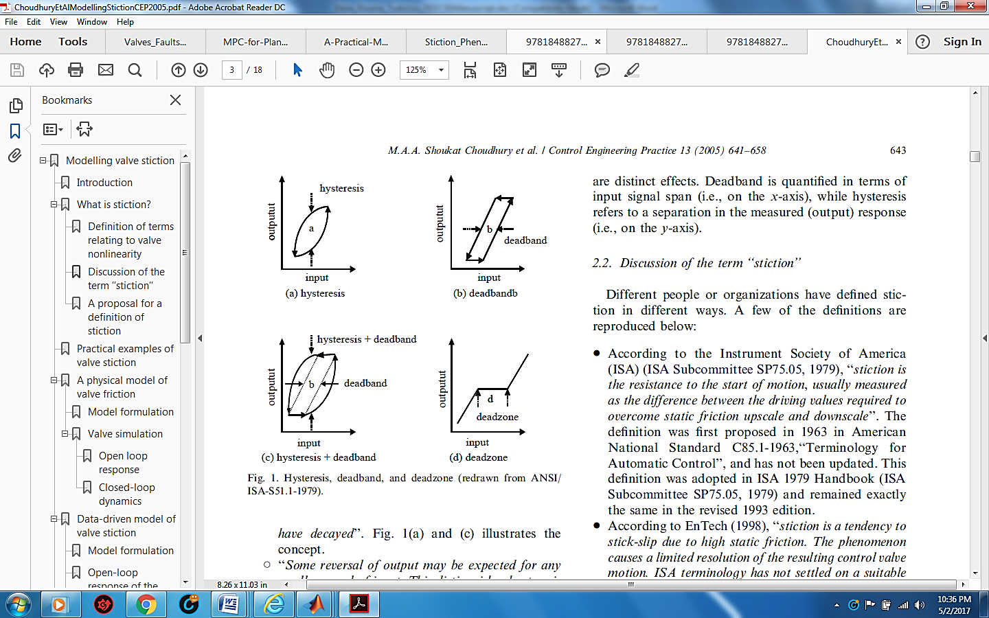Figure 1: The hysteresis, dead-band, and dead-zone valve nonlinearities (screenshot view [7], according to ANSI/ISA-S51.1-1979).

3. Dead-band: ‘‘In process instrumentation, it is the range through which an input signal may be varied, upon reversal of direction, without initiating an observable change in output signal’’, as is shown in Figure 1(b).

The dead-band is not a bijection relationship; it is characterized by an input-output phase lag, expressed in percent of its span [7]. Moreover, a combination of the effects of dead-band and the hysteresis may be met as a new nonlinearity in a control valve actuator, as is shown in Figure 1(c). “Some reversal of output may be expected for any small reversal of input. This distinguishes hysteresis from dead-band’’ [7].

4. Dead-zone: ‘‘It is a predetermined range of input through which the output remains unchanged, irrespective of the direction of change of the input signal’’, as is shown in Figure 1(d).

Unlike dead-band, the dead-zone doesn’t produce an input – output phase leg, so it is expressed by a bijective input-output relationship.

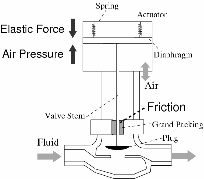Figure 2: The structure of the pressure control valve (snapshot view [8])

These definitions reveal that the term ‘‘backlash’’ specifically applies to the slack or looseness of the mechanical part when the motion changes its direction [7]. In addition, the above ANSI (ISA-S51.1-1979) definitions illustrated clearly in Figure 1 prove without doubt that hysteresis and dead-band nonlinearities have distinct effects on a control valve. More precisely, the dead-band can be quantified in terms of x-axis input signal span, while hysteresis refers to a separation in the y-axis measured (output) response [7]. The combined effects of the static and dynamic effects of the previous nonlinearities generate one of the most complex control valve nonlinearity known under the name of control valve stiction (static friction). Its input–output characteristics consist of four components: dead-band, stick-band, slip jump and the moving phase of a stiction faulty valve as is shown in Figure 3 [7].

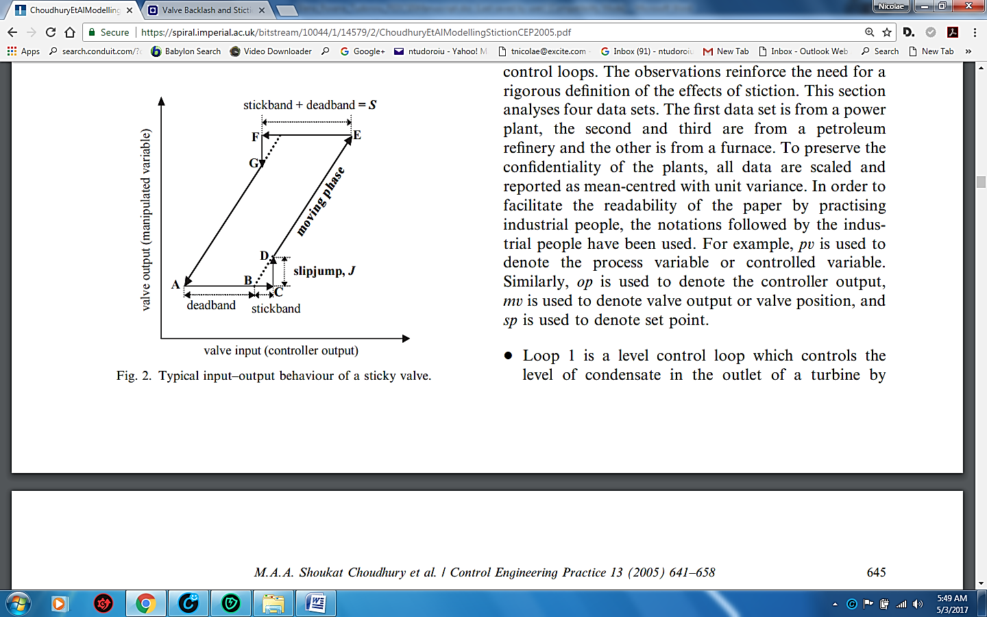Figure 3: The characteristics of a sticky faulty control valve (Screenshot view [7])

The behavior of a sticky faulty valve is completely described in [7] as ‘‘a property of an element such that its smooth movement in response to a varying input is preceded by a sudden abrupt jump called the slip-jump. Slip-jump is expressed as a percentage of the output span. Its origin in a mechanical system is static friction which exceeds the friction during smooth movement’’. In this description the dead-band and stick-band represent the behavior of the non-moving control valve, while its input keeps changing. The slip jump releases suddenly the potential energy stored in the control valve chambers due to its stem high static friction in order to balance the kinetic energy as the valve starts to move. More precisely, the magnitude of the slip jump is one of the main causes in generating the limit cyclic behavior by the control valve stiction [7]. Once the valve slips, it continues to move until it sticks again (e.g., in the point E from Figure 3), and during all this moving-phase was proved that the dynamic friction may be much lower than the static friction [7]. The definition of the stiction well illustrated in Figure 3 can be considered as a rigorous description of the effects of friction in a control valve.  Closing, these definitions will be very useful in the following sections to characterize the pattern features of the impact of several actuators nonlinearities in industrial control systems practice; under consideration will be the both continuous and discrete time state-space models of healthy and faulty open or feedback closed-loop control systems configurations. The healthy and faulty control systems responses from time domain will be converted in frequency domain by using different types of wavelet transforms that will be defined in the next section. Based on wavelet analysis in frequency domain will be extracted the matching pattern features that characterize each control valve nonlinearity under investigation.

3.       Wavelet Signals Processing Technique Approach

The signal processing approach is one of the most used techniques used in practice for signal analysis. It is focused on particular signal characteristics, dealing also with the effects of the “white” or “colored” noises that contaminate the useful signals, by using statistical methods, such as the signals correlation and autocorrelation functions, covariance and cross-covariance, power spectral density, likelihood, or the autoregressive-moving-average (ARMA) models [9]. Frequency analysis is suitable for detecting the signals that contain particular meaningful frequency information, very useful to be used for example to detect, diagnose and isolate the healthy or faulty behavior of the control systems as response to the effects of a particular actuator nonlinearity or sensor faults, known in the control system literature as fault detection and isolation (FDI) techniques [10].  In this paper work are extracted only some of the pattern features of the healthy or faulty responses corresponding to control valve (actuator) nonlinearities under investigation. The wavelet transform is useful to detect the abrupt changes (signals pattern features) in the faulty actuators or sensors.  It provides a useful set of time-scale or time-frequency domain tools and techniques to operate on a large range of signals [9]. The wavelet transform carries out a special form of analysis by shifting the original signal from the time domain into the time–frequency [11]. According to [11] “the idea behind the wavelet transform is to define a set of basic functions that allow an efficient, informative and useful representation of signals”, and first preliminary attempts to demonstrate the new theory based on the wavelet analysis started with the modeling of “a certain signal by a combination of translations and dilations of a simple, oscillatory function of finite duration, named wavelet “, and this technique is referred to as a continuous wavelet transform (CWT) [9]. In [11] also is mention that “Having emerged from advancement in time–frequency localization from the short–time Fourier analysis, the wavelet theory provides facilities for a flexible analysis as wavelets figuratively “zoom” into a frequency range. Moreover, the “wavelet methods constitute the underpinning of a new comprehension of time–frequency analysis”.  Based on CWT many other wavelet analysis techniques have been developed in the literature [9], among them, due to paper space limitation, only one of these it will be considered. Depending on the intended purpose, if low-frequency information is required then the wavelet analysis deals with long time intervals, otherwise it will deal with short time intervals when high-frequency information is preferred.  In the following we will give some definitions that can be of real interest for the readers in order to have a good insight on all these concepts related to wavelet transforms as well as their manipulation in signals analysis and processing.

CWT Definition 1: The continuous-time wavelet transform of one-dimensional real-valued function, -Hilbert space, measurable and square-integrable, i.e. , with respect to a wavelet function is defined as the sum over all time of the signal multiplied by scaled, shifted versions of function [9]:

where  represents the complex-conjugate of the “mother wavelet” , a  real or complex-valued continuous time function that must satisfy the following two conditions:

 is a function with zero-average:

, i.e. is a squared-integrable function, i.e.  .

A “mother wavelet” is a waveform for which the most energy is restricted to a finite duration [9], with the mention that there are an infinite number of the functions that candidate to be considered as a “mother wavelet”.

In Eq. (2) the variable s is a “scale” or “dilation” variable that performs  a stretching or compressing action on the “mother wavelet” while the variable u is referred as a “time shifting” or “translation” that delays or hastens the signal start.

  More precisely, the function  means that the mother wavelet is shifted over time with u units of time and s times dilated. Therefore the wavelet analysis is a powerful tool that provides a time-scale view of the signal under investigation.

then the  CWT of the continuous function can be expressed by a  the following convolution product (*):

Also, it is worth to emphasize that the result of applying CWT to a signal under investigation is a wavelet coefficient vector that is a function of scale and translation g(s, u). An interesting interpretation related to a wavelet coefficient vector is done in [9], stating that “each coefficient represents how closely correlated a scaled wavelet is with the portion of the signal which is determined by translation”.  The CWT coefficients are nothing else than time-scale view of the analyzed signal, and so the CWT is an important analysis tool capable to “offers insight into both time and frequency domain signal properties” [9].  The results of this interpretation lead to the following useful observations [9] that will be considered for developing the proposed wavelet signals processing and analysis strategy:

The higher scales correspond to the “most” stretched wavelets, furthermore “the more stretched the wavelet, the longer the portion of the signal with which is compared, and thus the coarser the signal patterns features measured by the wavelet coefficients”.

The “…coarser features called “approximations” providing basic shapes and properties of the  original signal under investigation correspond to low frequency components, whereas the low scale components capture the high frequency information, called “details”…”.

The main drawback of CWT is its computationally inefficiency due to the calculation of the CWT coefficients at every single scale with an impressive amount of work generating a huge bunch of data that must be stored in a considerable computer memory space. An alternative to the CWT is the discrete wavelet transform DWT, much more efficient and of high accuracy.  The DWT is based on the wavelet analysis at particular scales and translations that are power of two, such as 2, 4, 6, 16, and so on [9], [10]. In [9] is stated that “the approximations” of the signals under investigation “provide basic trends and characteristics of the original signals, whereas the details provide the flavor of the signal”, and the result of the applying DWT on the analyzed original signal is the so called wavelet decomposition around two key coefficient vectors, one of them is an “approximation” coefficient vector Ca, and other one is a “detail” coefficient vector Cd, representing “approximations” and “details”  of the original signals under consideration.  If the decomposition is repeated on the approximations in each stage, then the multiple stage DWT will break down the original analyzed signal into many successively lower resolution components, as is shown in [9], section 5.1.2, pp.79. According to [9] “at each stage, the approximation coefficient Ca represents the signal trend, and the detailed coefficient Cd   includes the   information on noise or nuance”.  The inverse process opposite to decomposition is the signal reconstruction by using an inverse discrete wavelet transform (IDWT).  More details about sample wavelet definitions known as Haar, Mexican Hat, Morlet and Daubechies wavelets are well documented in [10]. Using the MATLAB/SIMULINK   Wavelet and Processing Toolboxes will be implemented in real time the proposed  multifractal and multisignal 1-D wavelet analysis strategy following the guidelines from  [13], [14].

4.       Case Study: pH Neutralization Plant

For simulation purpose the experimental setup for the pH neutralization process and the dynamic model coefficients are the same as in [15]. The tank layout is shown in Figure 3.

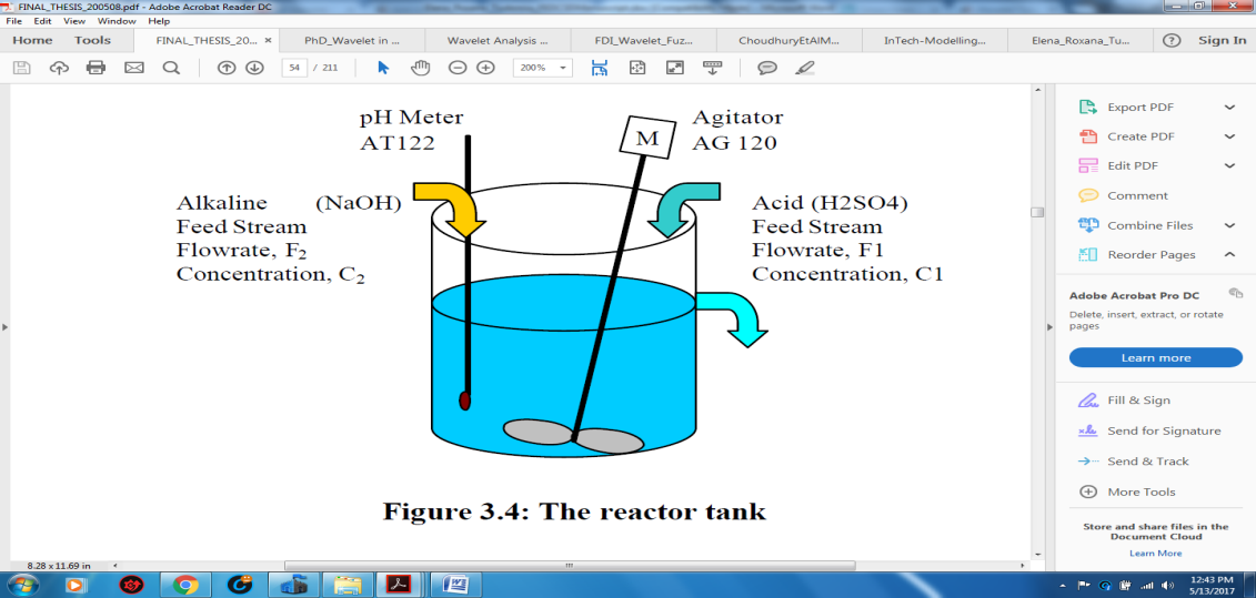Figure 4: The reactor tank layout (screen shot view [11], pp. 41, Section 4)

Of technical viewpoint as the piping and instrumentation diagram layout, the tank and the overall architecture we preferred the simplified representation shown in Figure 4 to Figure 7 reproduced from [11] for their simplicity and better insight. They are related to the same pH neutralization process, only the coefficients of the models make the difference due to the changes in reactors geometry, flow rates and concentrations of acid and alkaline reactants.

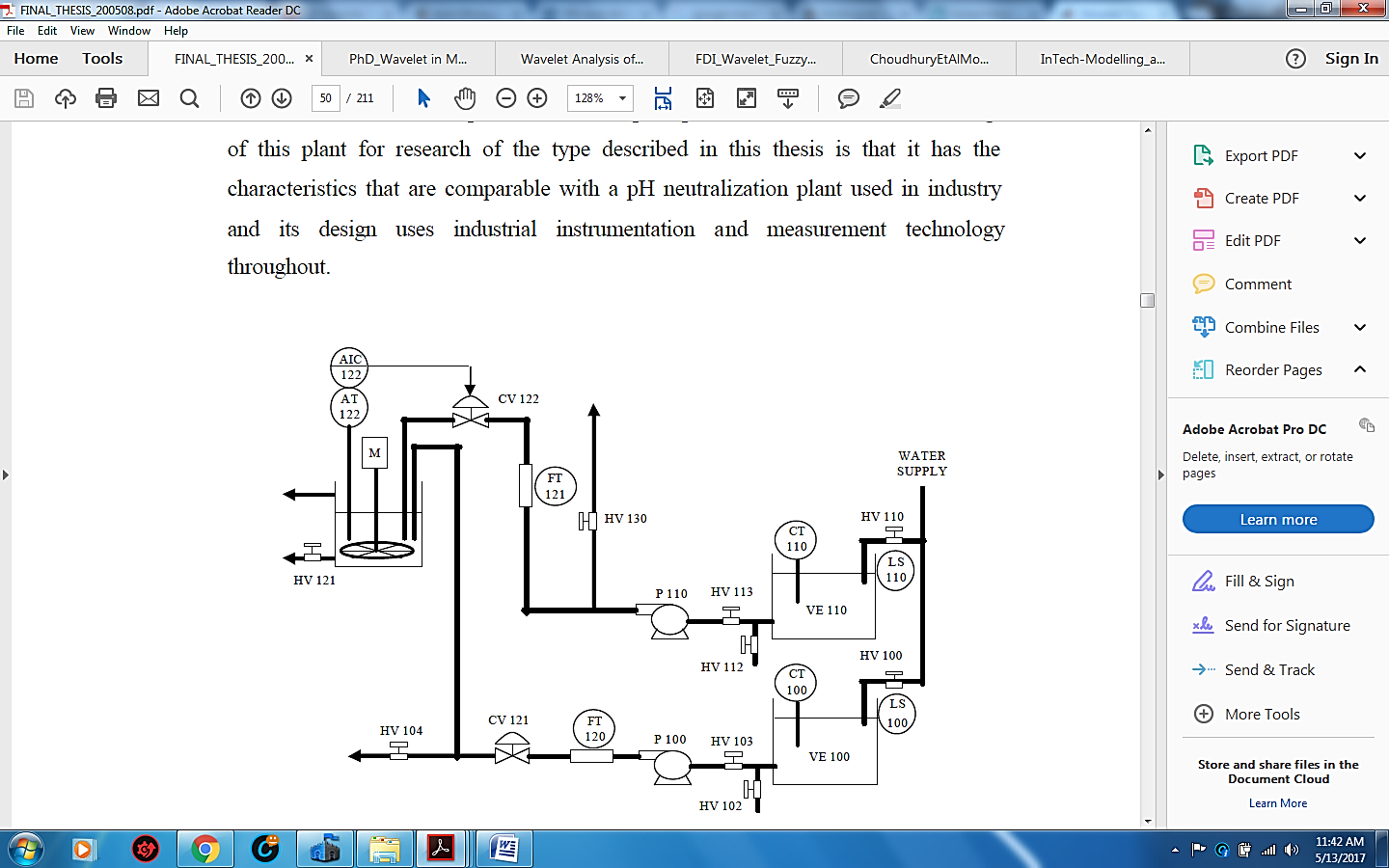Figure 5: Piping and Instrumentation Diagram of pH neutralization plant (screen shot view [11], pp. 37, Section 3)

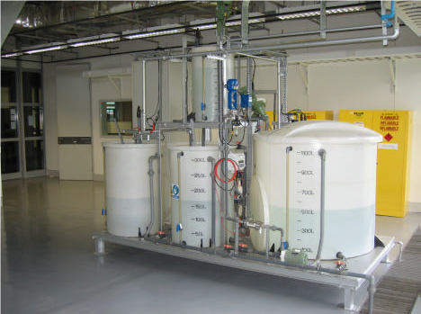Figure 6: The picture of the neutralization pilot plant (snapshot view [11], pp. 38, Section 3)

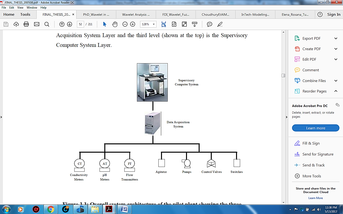Figure 7: Overall architecture of the pH neutralization pilot plant (screen shot view [11], pp. 39, Section 3)

In Figure 8 is shown the block scheme of the both control loops, i.e. pH concentration value, and level of the solution inside the neutralization reactor.

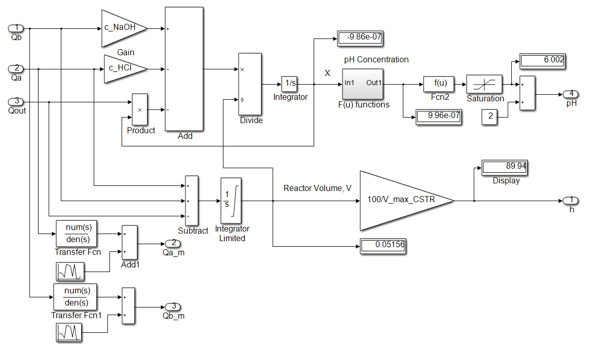Figure 8: The SIMULINK model of the solution level control inside of the neutralized reactor and pH control closed-loops [15]

In Figure 9 is shown the SIMULINK model of the pH- controller with a back-propagation windup reset to avoid the saturation of the integrator due to the saturation nonlinearity of the control valve actuator. In Figure 10 and Figure11 is shown in detail the PI level controller with a windup reset from the same raison as for PI pH-controller.

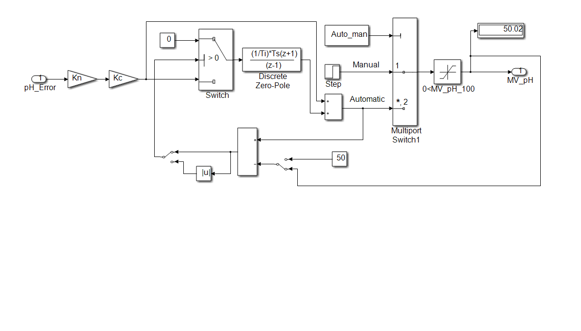Figure 9: The SIMULINK model of pH controller with windup integrator [15]

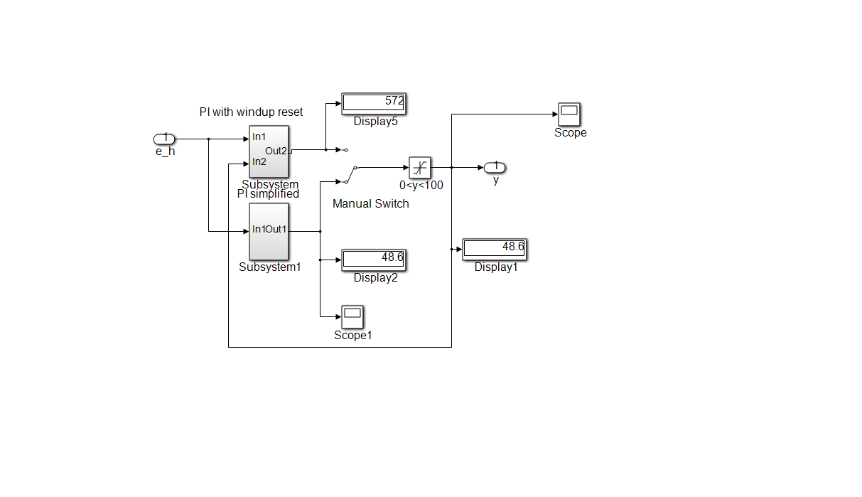Figure 10: The simplified SIMULINK model of the Level PI   Controller Block [15]

5.       MATLAB and SIMULINK Simulations Results in Time Domain

In this section we will present the simulation results of the control system performance in closed-loop, in time domain.

A.       Healthy Control System with Pump and Control Valve Actuator Enabled

The pH step response is shown in Figure 11, for which the input profile changes the initial step input from pH12 after 5000 seconds (1h23min) to standardized pH8, the total simulation time taking 10000 seconds (2h46min).

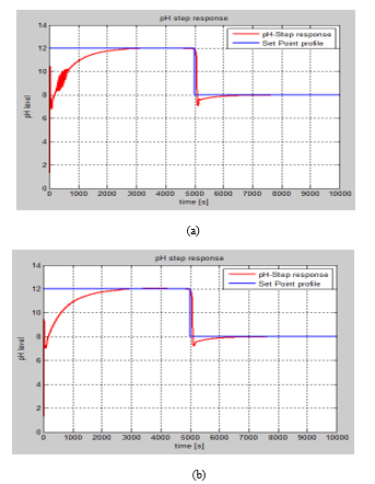Figure 11: The step response of the pH concentration of the neutralized solution inside the reactor.

Legend: a. Control valve enabled

1.   Pump enabled

From performance analysis prospective the simulation results reveal a very accurate performance for the both PI controllers with windup reset. All these simulation results are carried out in a MATLAB SIMULINK simulation environment based on the SIMULINK model of the overall control system structure with the both feedback closed-loops, shown in Figure 12, similar as is developed in [16]. The step response of the level of neutralized solution inside the reactor controlled by a PI controller with windup reset is shown in Figure 12.  In Figure 13 is presented the step response of the neutralized solution level inside the reactor. The controller efforts for pH and level are shown in Figure 14 and Figure 15.

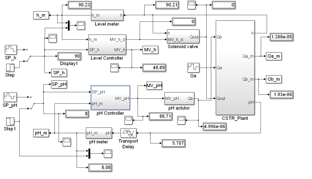Figure 12: The SIMULINK model of the overall closed-loop control system [15]

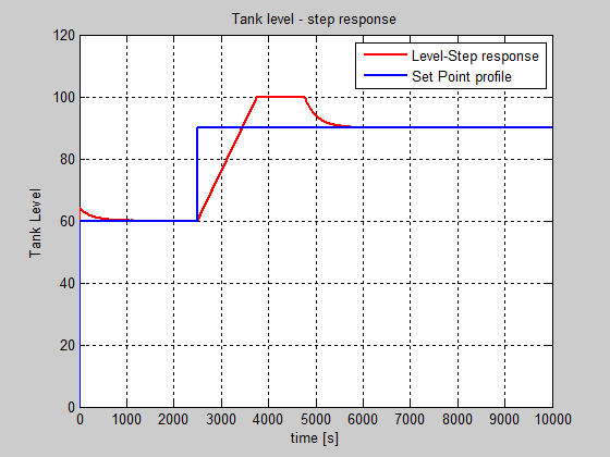Figure 13: The step response of the neutralized solution level inside the reactor.

Let us now to consider the presence of a time delay in the pH control loop, i.e. pH sensor transmits the pH measured value to the input of the pH controller with certain amount of transport delay, let say for example 10 seconds, same value as is the time constant of the pH controller, you can see in Figure 16 that the pH control loop starts to oscillate at beginning of the simulations reaching the target steady-state for a while (2000 seconds) since after the first switching moment in setting point the closed-loop reaches the limit of stability around the second target setting point, thus the controller becomes now inadequately. In this case is required a simple adaptive Smith-Predictor control structure for controlling time-delay systems, such is developed in [16].

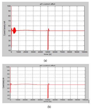Figure 14:  The SIMULINK simulations of the pH controller effort in closed-loop

 Legend: a. Control valve enabled

1. Pump enabled

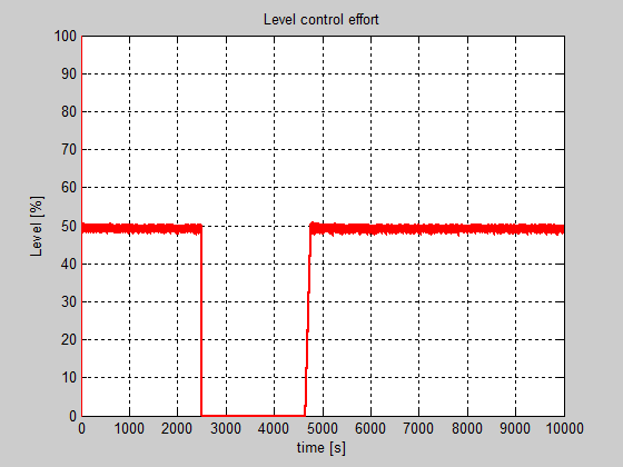Figure 15:  The SIMULINK simulations of the controller level effort in closed-loop

A considerable control effort of pH controller can be seen in this case in Figure 17. During these simulations no interferences between the two controls loops were noticed, thus the level control loop still remains very accurate.

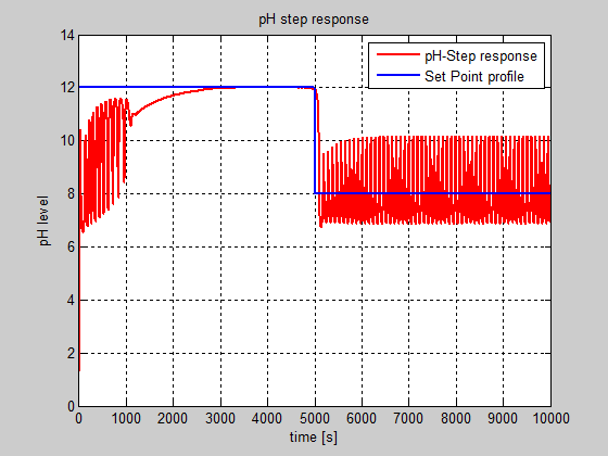Figure16:  The SIMULINK simulations of the pH concentration in closed-loop with 10 seconds time delay in signal transmission

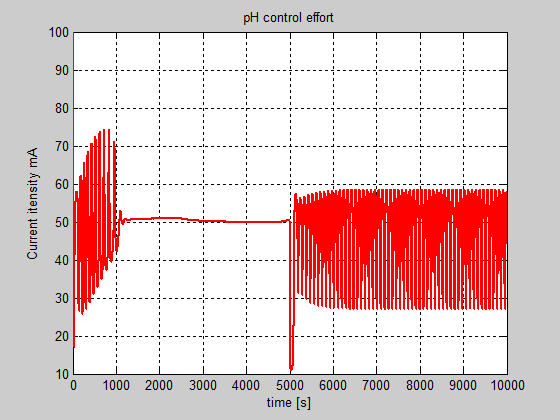Figure 17:  The SIMULINK simulations of pH controller effort in the     presence of 10 seconds time delay in signal transmission

B.       Faulty Control System with Control Valve Actuator Enabled

In this subsection we analyze the impact of control valve actuator nonlinearities on the overall control system performance.

1. Backlash control valve actuator nonlinearity shown in Figure 18 with dead-band width = 0.7, SIMULINK model.

In Figure 19 is shown the impact of the control valve backlash nonlinearity on the pH closed-loop control for the same set point input profile setup and the same tuning values for the pH controller parameters as for healthy control system structure. In this case the overall performance of pH control closed-loop degrades significantly. This is the first pattern feature extracted from measured pH output signal in time domain that will be analyzed in frequency domain by using a fractal analysis based on the wavelet transforms. The control effort is considerable also in this case, as is shown in Figure 20.

2. Coulomb and Viscous friction nonlinearity in control valve actuator shown in Figure 21 with the coefficient of viscous friction (gain) = 0.1, the Coulomb friction value (offset) = 1, SIMULINK model.

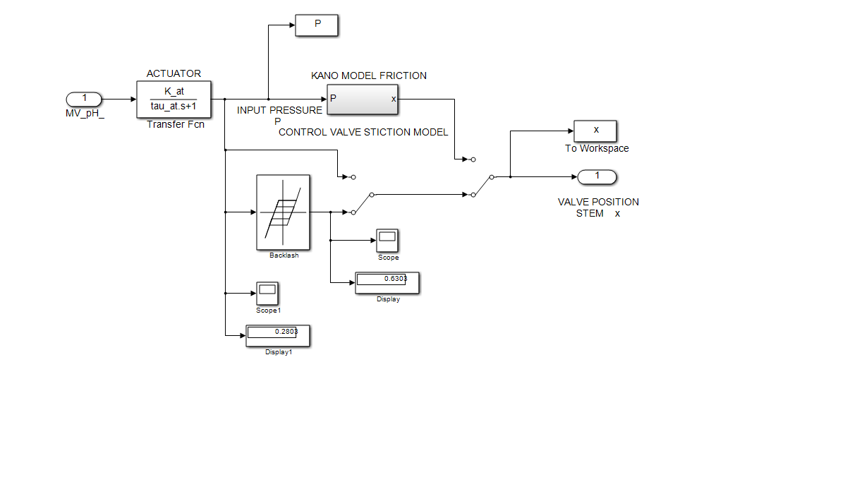Figure 18:  SIMULINK model of the control valve actuator with backlash nonlinearity (dead-band width = 0.7)

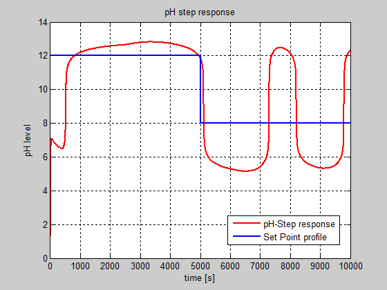Figure 19: The impact of backlash control valve actuator nonlinearity on the pH evolution in closed-loop (dead-band width = 0.7, SIMULINK model).

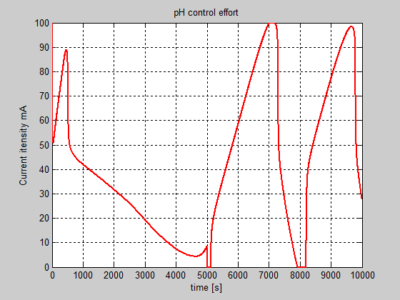Figure 20:  The pH control effort in the presence of backlash nonlinearity in the control valve actuator integrated in the pH control closed-loop (dead-band width = 0.7).

3. Dead-zone nonlinearity in control valve actuator shown in Figure 23 with a symmetric dead-zone width = 1, SIMULINK

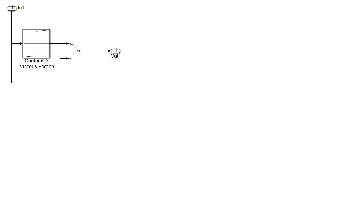Figure 21: SIMULINK model of the control valve actuator with Coulomb and Viscous friction nonlinearity, SIMULINK model

Similar, compared to backlash nonlinearity case the overall performance of pH control closed-loop degrades drastically, as is shown in Figure 22. This is the second pattern feature extracted from measured pH output signal in time domain that will be analyzed in frequency domain by using a fractal analysis based on the wavelet transforms.

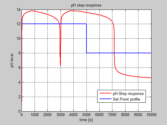Figure 22: The impact of Coulomb and viscous friction nonlinearity of control valve actuator on the pH evolution in closed-loop (Coefficient of viscous friction (gain) = 0.1, the Coulomb friction value (offset) = 1, SIMULINK model).

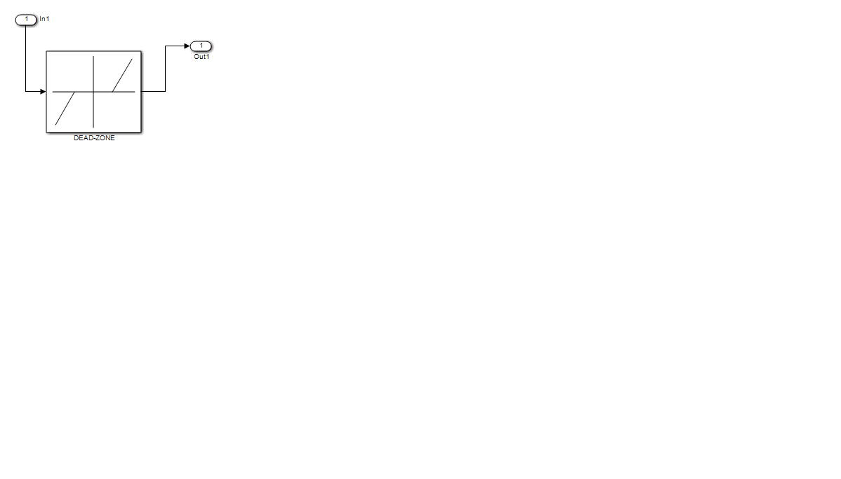Figure 23 SIMULINK model of the control valve actuator with Dead-zone nonlinearity, SIMULINK model (dead-zone width =1)

The impact of dead-zone nonlinearity on the overall performance is shown in Figure 24. This is the third pattern feature extracted from measured pH output signal in time domain that will be analyzed in frequency domain by using a fractal analysis based on the wavelet transforms.

Figure 24: The impact of Dead-zone nonlinearity of control valve actuator on the pH evolution in closed-loop (dead-zone width = 1, SIMULINK model).

4. Saturation nonlinearity in control valve actuator shown in Figure 25 with superior limit = 0.5 [Pa], and the inferior limit = 0[Pa], SIMULINK model.

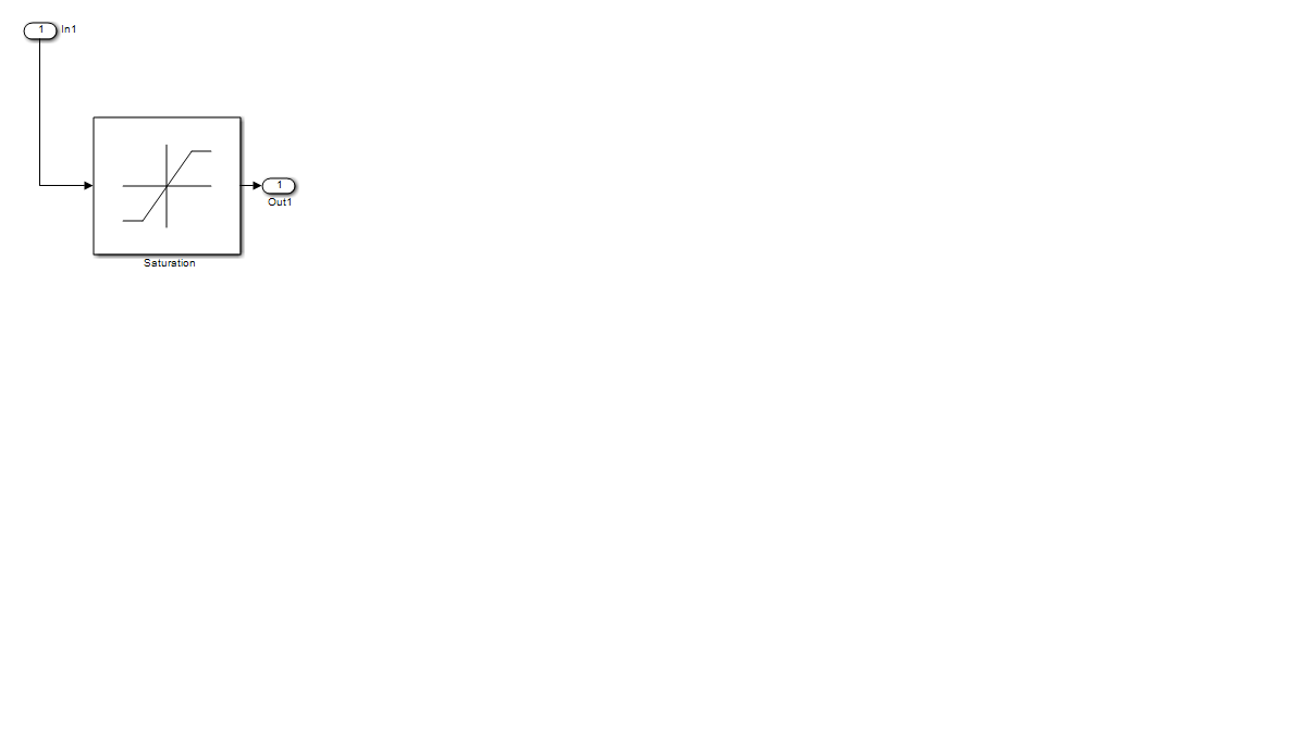Figure 25: SIMULINK model of the control valve actuator with saturation nonlinearity, SIMULINK model

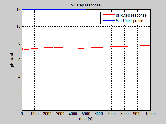Figure 26: The impact of saturation nonlinearity of control valve actuator on the pH evolution in closed-loop (dead-zone width = 1, SIMULINK model).

6.       Multisignal 1-D Wavelet Analysis – MATLAB Simulations Results

1-D Multisignal Definition 2: A 1-D multisignal is a set of 1-D signals of same length stored as a matrix organized rowwise (or columnwise) [14]. In the proposed case study all the signals are stored in a matrix with two rowwises, in a first row is stored the healthy signal and in second one is stored the corresponding faulty signal representing the impact of each actuator nonlinearity on the overall performance of healthy control system.  The purpose of this section is to make a wavelet analysis of the 1-D multisignal set containing all the nonlinearities described in the previous section. How you will see the wavelet analysis is a precious analysis tool to denoise, compress and cluster different representations or their simplified versions. In first step a deeply analyze is made for all  the signals collected in the previous section from the closed-loop control system, and then we will find some representations and also simplified versions for  these signals by reconstructing their approximations  at given levels,  denoising and compressing them.

Denoising and compressing are two of the main applications of wavelets, often used as a preprocessing step before clustering [14]. The last step performs several clustering strategies and compares them. It allows summarizing a large set of signals using sparse wavelet representations. In Figure 27 you get an overall image about the impact of all control valve actuator nonlinearities on the closed-loop performance of the neutralization control system discussed in previous section.

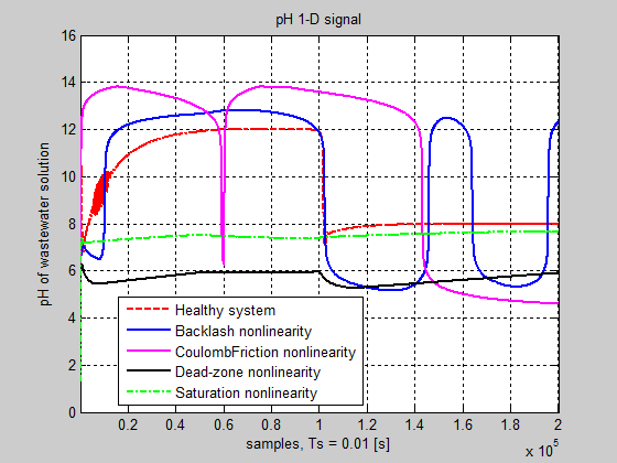Figure 27: The impact of the control valve nonlinearities on the closed-loop performance of pH control system

The same overall image you can get as more attractive in a 3-D representation of all these nonlinearities including also the healthy control system, as a reference for  the severity of each impact, is offered in Figure 28, The 3-D representation is preferred  in addition to highlight  the periodicity of the multisignal.

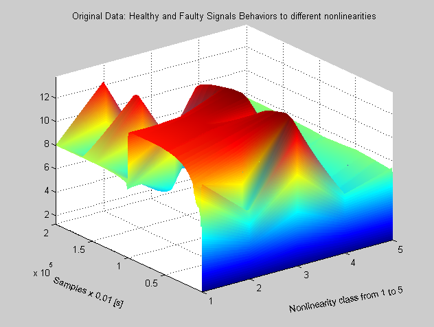Figure 28: The 3-D representation of the impact of several control valve nonlinearities, on the closed-loop control system performance.

In 3-D representation each nonlinearity impact can be seen more clearly. In Figure 29 is shown the row decomposition of the multisignal related to the following fields of the generated structure in MATLAB R2013a:

dirDec: ‘r’ (row decomposition)         Level of decomposition: 7         wname: ‘sym4′(near symmetric wavelet, as is shown                      in Figure 29)          dwtFilters: [1×1 struct]         dwtEXTM: ‘sym’         dwtShift: 0         dataSize: [35 1440]            ca: [35×18 double]            cd: {1×7 cell}

4

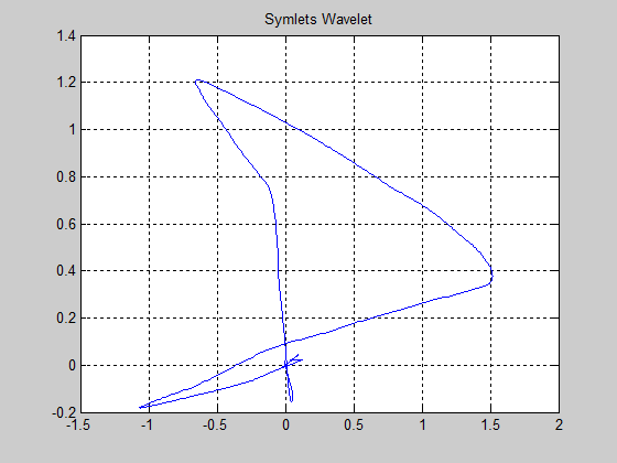Figure 29: The symlet wavelet (“sym4’) representation

MATLAB Wavelets Toolbox offers you more facilities to get information about all these wavelets functions using the MATLAB command waveinfo(‘name’), where ‘name’ is the assigned short name for the wavelets families such as ‘sym’, ‘morl’, ‘haar’, ‘db’, and so on.  The reconstruction of the approximations at level 7 for each row signal is shown in Figure 30.  The signals reconstructed are also compared in the same graph to the original signals. Furthermore, to get a better insight about the control valve nonlinearities under investigation in Figure 31 the signals are split in two groups, in the first group the healthy signal, the backlash and Coulomb viscous friction, and in second group the last two nonlinearities, control valve dead-zone and saturation.

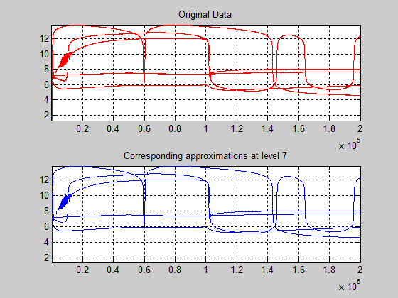Figure 30: The original signals and the reconstruction of the approximations at level 7 for each row.

The top plot shows all the original signals and the bottom one shows all the corresponding approximations at level 7. As it can be seen, the general shape is captured by the approximations at level 7, but sometimes some interesting features are lost, as for example, the bumps at the beginning and at the end of the signals could disappear.

In order to perform a more subtle simplification of the multisignal preserving these bumps a denoise operation of  the multisignal is useful. The denoising procedure is performed in MATLAB R2013a following three steps, namely [15]:

• Decomposition: First is required to select a wavelet function and to set up the level of its decomposition N, and then compute the wavelet decompositions of the signals at level N.
• Thresholding: For each level from 1 to N and for each signal, a threshold is selected and thresholding is applied to the detail coefficients.
• Reconstruction: Compute wavelet reconstructions using the original approximation coefficients of level N and the modified detail coefficients of levels from 1 to N.

If a slightly change will be made at the level of decomposition by changing N from 7 to N = 5 in Figure 32 can be seen similar results as in Figure 30, but now the quality of the results is better since the bumps at the beginning and at the end of the signals are well recovered. Conversely, in the same figure the residuals look like a noise except for some remaining bumps due to the signals. Furthermore, the magnitude of these remaining bumps is of a small order.

In Figure 33 are shown the results of the signals compression operation that follows the same three steps as in denoising case, a slightly difference in terms of the procedure is found only in step 2 that where  two compression approaches are available [15]:

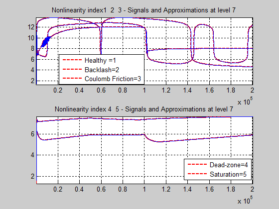Figure 31: The signals and approximations at level 7 of row decomposition split in two groups

In the first approach the wavelet signals are expanded and keep the largest absolute value coefficients; in this case, a global threshold, a compression performance, or a relative square norm recovery performance can be set [15]. Therefore, for this approach only a single signal-dependent parameter needs to be selected. In the second approach a determined level-dependent threshold is chosen visually. The compression performance can be evaluated by calculating the corresponding densities of nonzero elements, as is shown in Figure 34.

For all the control valve nonlinearities under investigation that causes faulty signals, as well as for healthy signal, the percentage of required coefficients to recover 99% of the energy is the same, approximately   0.75%.  This is one of the stronger wavelets features to prove a high capacity to concentrate all signal energy in few coefficients [15].

The last step is the clustering of the wavelets signals that offers a convenient procedure to summarize a large set of signals using sparse wavelet representations (with small number of elements). In Figure 35 the wavelets signals are clustered by 3. The first one is related to  the Coulomb viscous friction  nonlinearity  of the control valve, the second cluster is related to  the  healthy and baclash nonlinearity, and the third cluster is related to dead-zone and saturation nonlinearities.

The partition of all three clusters can be seen in Figure 36.

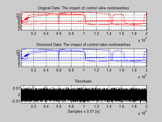Figure 32: The original signals, their approximations at level 5 of row decomposition, and the residuals.

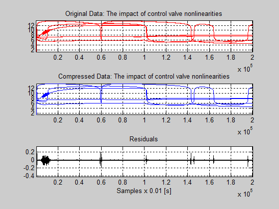Figure 33:  The original and compressed signals and the  corresponding residuals

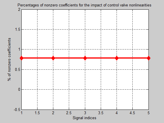Figure 34: The percentage of nonzero coefficients for all the control valve nonlinearities wavelet signals

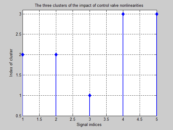Figure 35: The three clusters of  the wavelets signals correspondin to the healthy and control valve nonlinearities

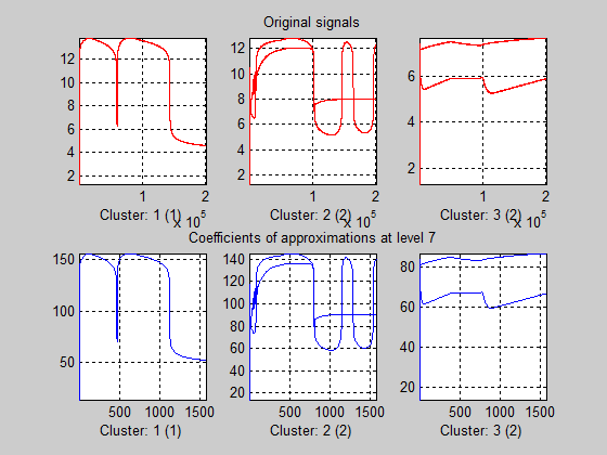Figure 36: The partition of each cluster in healthy and faulty control valve signals

7.       1-D Wavelet Analysis as a Detection Tool of the Actuators Faults in Control Systems

In this section we investigate how to use the 1-D wavelet analysis to detect changes in the variance of a process control.

 Changes in signal variance provide precious information anytime when something fundamental has changed about the data-generating mechanism that is basically the main idea of implementation for Fault Detection Diagnosis and Isolation (FDDI) strategies capable for detection, diagnosis and isolation of the faults that occur in actuators and sensors in a lot of control systems applications. In this section we investigate the effectiveness of using the 1-D wavelet analysis to detect some anomalies caused by malfunctioning of the equipment or different control system parts, especially actuators and sensors more likely prone to the errors.  Encouraged by the experience and the preliminary results obtained in the control systems field, such as modeling and process identification, state estimation and FDI control strategies,   a new FDI approach based on signal processing analysis to improve the accuracy, robustness and implementation design of these techniques is a big challenge. For simulation purpose we analyze only the impact on the overall closed-loop control performance of two control valve actuator nonlinearities, namely the backlash and Coulomb viscous friction, met frequently in the control industrial applications, as is shown in the Figures 37 and 38. In the Figure 37 is shown the SIMULINK model of the backlash nonlinearity that occurs often in control valve actuator, with the injection mechanism of the related fault at the instant t_{fault_injection} = 7000 seconds. The set point input profile changes also at the instant t_SP1=5000 seconds, from pH12 to pH8. Similar, in the Figure 38 is shown the SIMULINK model of the Coulomb viscous friction control valve nonlinearity and the injection mechanism of the related fault. Similar, in Figure 39 is presented the mechanism of generating the values for the backlash width using the clock block and if-then with separate triggered action block.

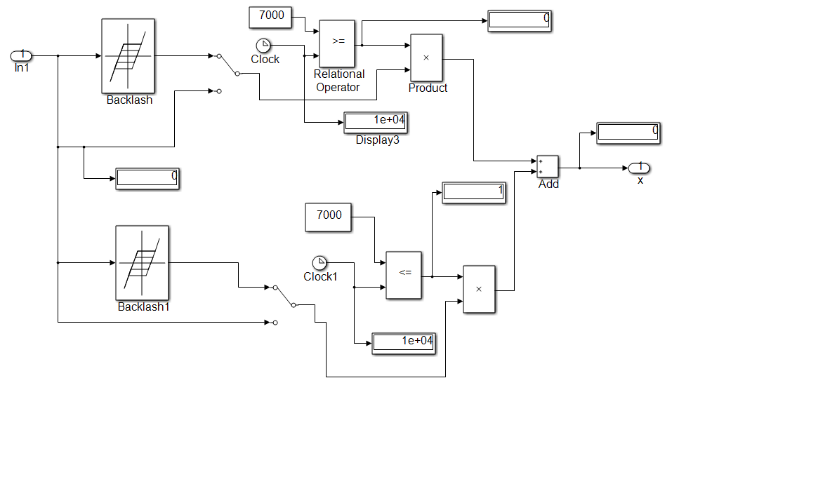Figure 37: The SIMULINK model of backlash nonlinearity in the  faulty control valve and  the injection mechanism

In the Figures 40 and 41 are shown the injection instant of the both faults (backlash and Coulomb viscous friction), and also the faulty behavior of the control system after this instant.

 Precious information about the time detection and the severity of the faults in each case is provided by the residuals defined as a difference between the healthy signal output (free fault) of the control system and faulty signal output, as is shown in Figure 42 and 43.

Figure 38: The SIMULINK model of Coulomb viscous friction  nonlinearity in the  faulty control valve and  the injection mechanism.

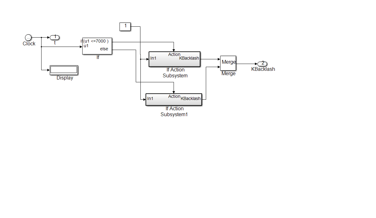Figure 39: The SIMULINK model of   generating the width  values for backlash nonlinearity in the  faulty control valve required in  the injection mechanism.

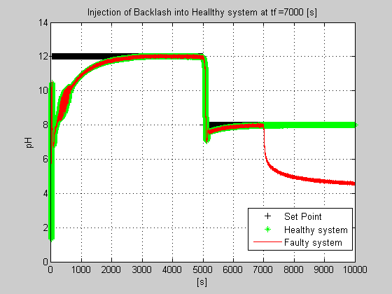Figure 40: The MATLAB simulation results for healthy and faulty behavior caused by the backlash nonlinearity in the  control valve actuator

Amongst the wavelets families functions the Morlet wavelet function shown in Figure 44 is suitable for continuous analysis using a continuous wavelet transform (CWT) [10], [17].  There is no scaling function associated with the Morlet wavelet. In many signal processing applications the Daubechies wavelet family functions are most used, especially for discrete wavelet transforms (DWT) [19].  To display detailed information about the Daubechies’ least asymmetric orthogonal wavelets is used the MATLAB command waveinfo(‘sym’). To compute the wavelet and scaling function (if available), use wavefun( ):

             [psi,xval] = wavefun(‘morl’,10);

             plot(xval,psi); title(‘Morlet Wavelet’);

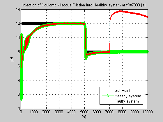Figure 41: The MATLAB simulation results for healthy and faulty behavior caused by the Coulomb viscous  friction in the  control valve  actuator

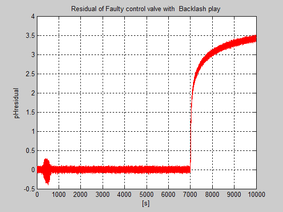Figure 42: The MATLAB simulation results for output control system residual caused by the  backlash nonlinearity in the  control valve actuator

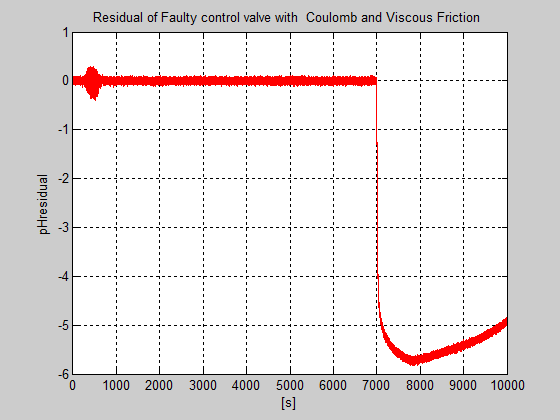Figure 43: The MATLAB simulation results for output control system residual caused by the  Coulomb viscous friction in the  control valve actuator

For wavelets associated with a multiresolution analysis can be computed both the scaling function and wavelet. The following MATLAB code returns the scaling function and wavelet for the Daubechies’ extremal phase wavelet with 4 vanishing moments [17], as is shown in Figure 45:

[phi,psi,xval] = wavefun(‘db4’,10);

subplot(211);

plot(xval,phi);

title(‘db4 Scaling Function’);

subplot(212);

plot(xval,psi);

title(‘db4 Wavelet’);

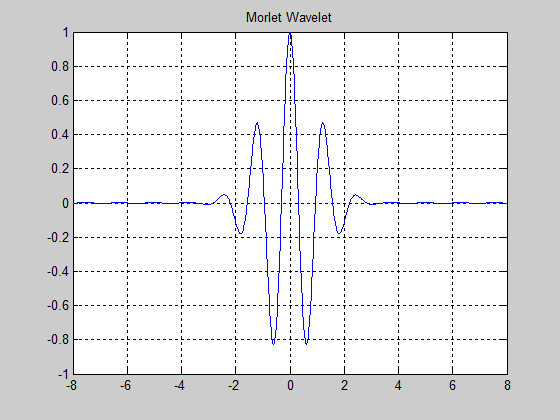Figure 44: The Morlet wavelet function representation with 10 vanishing moments

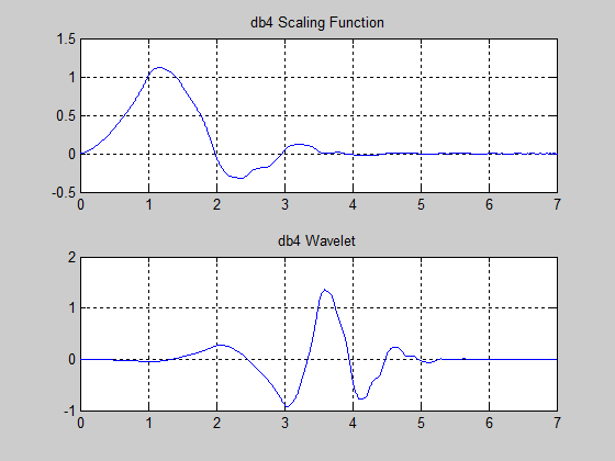Figure 45: The Daubechies’ extremal phase wavelet with 4 vanishing moments

In discrete wavelet analysis, the analysis and synthesis filters are of more interest than the associated scaling function and wavelet. For filter design and implementation you can use wfilters( ) to obtain the analysis and synthesis filters. For example, in order to obtain the decomposition (analysis) and reconstruction (synthesis) filters for the Bspline biorthogonal wavelet is required to  specify 3 vanishing moments in the synthesis wavelet and 5 vanishing moments in the analysis wavelet with the following MATLAB cod lines to generate and to  plot the filters’ impulse responses, very useful in this section for fault detection based on the wavelets filters analysis and synthesis (Low Pass Filters and High Pass Filters, used for low frequencies and high frequencies signals filtration respectively) [17]:

[LoD, HiD, LoR, HiR] = wfilters(‘bior3.5’);

subplot(221);

stem(LoD);

title(‘Lowpass Analysis Filter’);

subplot(222);

stem(HiD);

title(‘Highpass Analysis Filter’);

subplot(223);

stem(LoR);

title(‘Lowpass Synthesis Filter’);

subplot(224);

stem(HiR);

                                 title(‘Highpass Synthesis Filter’);

The simulation results are shown in Figure 46.

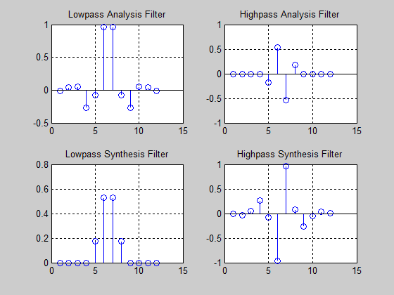Figure 46: The Daubechies’ extremal phase wavelet with 4 vanishing moments

The Daubechies wavelets (dbN) are the Daubechies’ extremal phase wavelets, for which N refers to the number of vanishing moments. These filters are also referred to in the literature by the number of filter taps, which is 2N [17], [21].

The Symlet wavelets (symN) are also known as Daubechies’ least-asymmetric wavelets. The symlets are more symmetric than the extremal phase wavelets. In symN, N is the number of vanishing moments. These filters are also referred to in the literature by the number of filter taps, which is 2N [17], [21].To obtain a survey of the main properties of this family, you must enter waveinfo(‘bior’) at the MATLAB command line. More precisely, the orthogonal and biorthogonal filter banks are arrangements of lowpass, highpass, and bandpass filters that divide the signals data sets into subbands [17], [21]. If the subbands are not modified, these filters enable perfect reconstruction of the original data. In most applications, the data are processed differently in the different subbands and then reconstruct a modified version of the original data. Orthogonal filter banks do not have linear phase. Biorthogonal filter banks do have linear phase [17], [21]. The wavelet and scaling filters are specified by the number of the vanishing moments, which allows removing or retaining polynomial behavior in the signals data sets. Furthermore, lifting allows designing perfect reconstruction filter banks with specific properties. In order to obtain and use the most common orthogonal and biorthogonal wavelet filters can be used Wavelet Toolbox™ functions [17].  The design of custom perfect reconstruction filter bank can be performed through elementary lifting steps. In addition, can also be added your own custom wavelet filters. However, by using the wavelet filter bank architecture depicted in Figure 47 it is possible to obtain residues that change in a noticeable manner in order to offer precious information about the time detection of the faults and its severity [19, 20]. The subband model is suggested in [19] of the form:

where s is an integer number and a, b are real numbers. In [19] is used the ‘db8’ wavelet for wavelet filter bank design of level 3 decomposition [19] for a  Single-Input Single-Output (SISO) plant  extended in [20] for a Multivariable (MIMO) plant. A wavelet based-frequency subband analytical redundancy scheme to calculate the residuals for different faults is shown in Figure 48, and used for wavelet filter bank synthesis and analysis of level 3 decomposition in [19, 20] , and also in our case study. In this scheme G(z) and H(z) represent the z-transforms of the low pass filter (LPF) and high pass filter (HPF) respectively.  A two-channel critically sampled filter bank filters the input signal using a lowpass and highpass filter [21].  The subband outputs of the filters are downsampled by two to preserve the overall number of samples. To reconstruct the input, upsample by two and then interpolate the results using the lowpass and highpass synthesis filters. If the filters satisfy certain properties, a perfect reconstruction of the input is achieved [21].  In Figure 49 is proved this perfect reconstruction by representing in the same graph the original faulty pH output signal (in the top) and the reconstruction faulty ph waveform response.

Figure 47:  Original wavelet analytical redundancy architecture for (a) input-output and (b) output-output consistency (snapshot view from [19], [20])

At each successive level, the number of scaling and wavelet coefficients is downsampled by two so the total number of coefficients is preserved. In order to obtain the level three DWT of the pH faulty signal is using the ‘sym4’ orthogonal filter bank, using the MATLAB code line [21]:

                           [C,L] = wavedec(wecg,3,’sym4′);

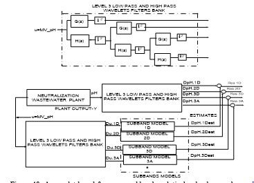Figure 48: A wavelet based-frequency subband analytical redundancy scheme (suggested in [19, 20])

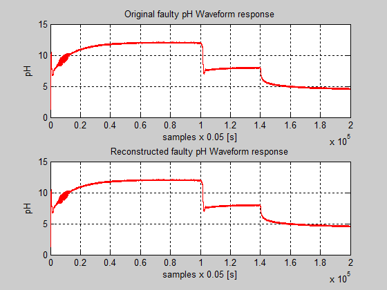Figure 49:  The original and reconstruct pH faulty signals

The number of coefficients by level is contained in the vector L. The first element of L is equal to 256, which represents the number of scaling coefficients at level 3 (the final level). The second element of L is the number of wavelet coefficients at level 3. Subsequent elements give the number of wavelet coefficients at higher levels until the final element of L is reached. The final element of L is equal to the number of samples in the original signal. The scaling and wavelet coefficients are stored in the vector C in the same order. In order to extract the scaling or wavelet coefficients, the MATLAB commands appcoef ( ) or detcoef.( ) can be used. All the wavelet coefficients are extracted in a cell array and final-level scaling coefficients [21]. In the Figures 50 and 51 are shown all these coefficients for faulty pH signal caused by backlash nonlinearity and for healthy pH signal (free faults) respectively.

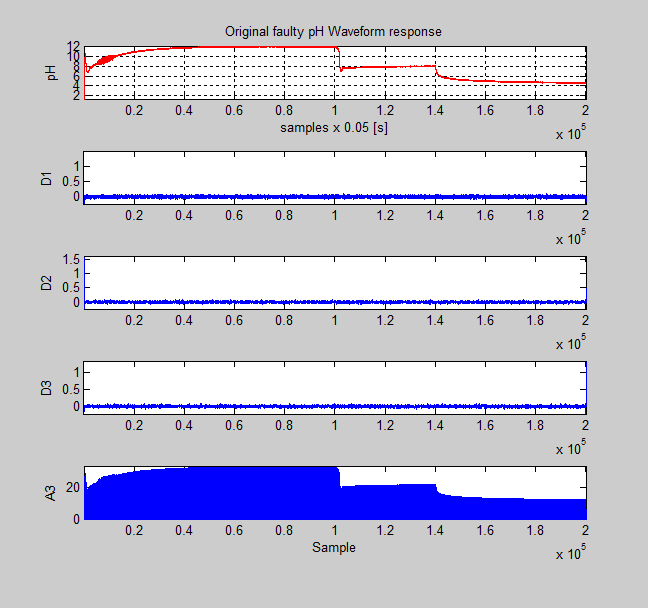Figure 50: The detailed vectors coefficients D1, D2, D3 and approximation vector coefficients A3 for faulty pH signal caused by the backlash in control valve actuator.

The residuals of the detailed coefficients Res1D, Res2D, Res3D and also of the approximation coefficients Res3A are shown in the Figures 52 until 55. All these figures reveal a good detection of the fault injection instant, and also provide useful information about the fault severity, as is shown in Figure 55. The residuals for detailed vectors coefficients are almost zero if the noise will be filtrated. Similar, for the second nonlinearity in the control valve actuator the detection procedure of the faults is the same. The simulation results are shown in Figures 56 until 61.

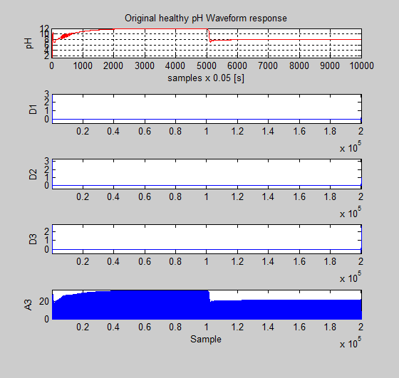Figure 51: The detailed vectors coefficients D1, D2, D3 and approximation vector coefficients A3 for healthy  pH signal

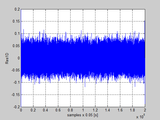Figure 52: The residual of the detailed vector coefficients Res1D

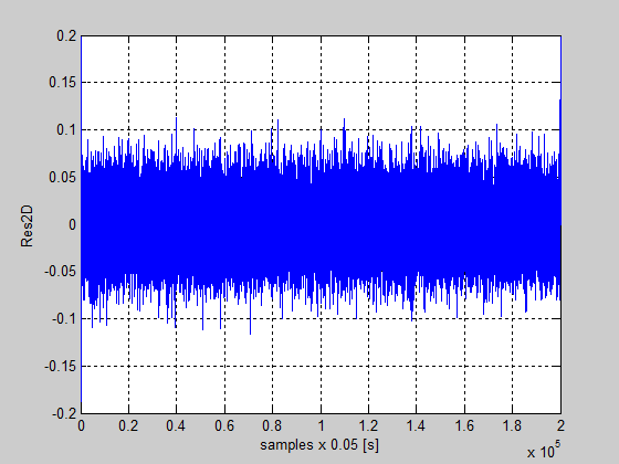Figure 53: The residual of the detailed vector coefficients Res2D

Figure 54: The residual of the detailed vector coefficients Res3D

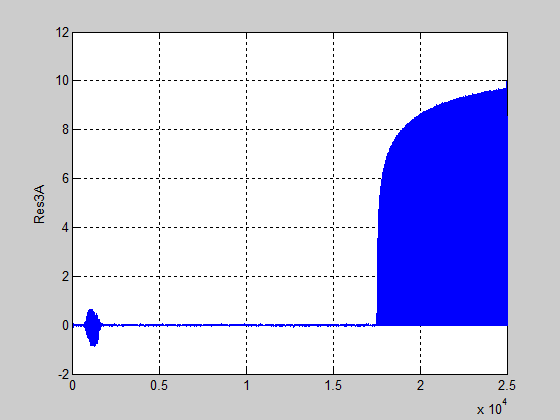Figure 55: The residual of the approximation vector coefficients Res3A

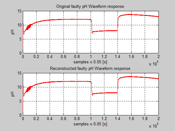Figure 56:  The original and reconstruct pH faulty signals caused by a Coulomb viscous friction in the control valve actuator.

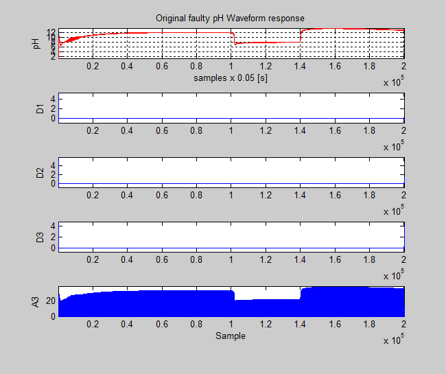Figure 57: The detailed vectors coefficients D1, D2, D3 and approximation vector coefficients A3 for faulty pH signal caused by the Coulomb viscous friction  in control valve actuator.

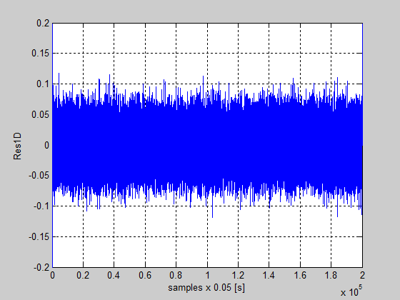Figure 58: The residual of the detailed vector coefficients Res1D

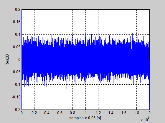Figure 59: The residual of the detailed vector coefficients Res2D

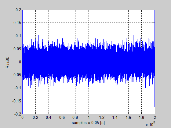Figure 60: The residual of the detailed vector coefficients Res3D

8.       Conclusions

In this research paper we open a new research direction in control systems applications field by performing a lot of investigations on the use of multisignal 1-D wavelet analysis to improve the accuracy, robustness, the design and the implementation in real-time of FDI techniques. These investigations are performed on the particular case study, mainly chosen to evaluate the impact of the uncertainties and the nonlinearities of the sensors and actuators on the overall performance of the control systems, namely a neutralization of wastewater plant, in an attractive MATLAB SIMULINK simulation environment. The preliminary simulation results are encouraged and extensive investigations will be done in future work to extend the applications area.  The 1-D wavelet analysis proved its effectiveness as a useful tool for signals processing, design and analysis based on wavelet transforms found in a wide range of control systems industrial applications. Based on the fact that in the real life there is a great similitude between the phenomena, we are motivated to extend the applicability of these techniques to solve similar applications from control systems field, such is done in our research work.

Conflict of Interest

The authors declare no conflict of interest.

Figure 61: The residual of the approximation vector coefficients Res3A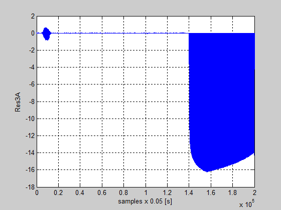

1. C.D. Bocaniala, J. Sa da Costa, and R. Louro, “A fuzzy classification solution for fault diagnosis of valve actuators”, Lecture Notes in Artificial Intelligence (Subseries of Lecture Notes in Computer Science book series, LNCS, Springer, Berlin, Heidelberg), vol.2773,Vasile Palade, Robert J. Howlett, and Lakhimi Jain (Eds.), pp. 741-747, 2003.
2. N.Tudoroiu, M.Zaheeeruddin,”Fault detection and diagnosis of the valves actuators in HVAC systems, using frequency analysis”, International Conference on Industrial Electronics and Control Applications, ICIECA 2005, 4 pages, Quito, 29 Nov.-2 Dec. 2005.
3. D. Düstegör, E. Frisk, V. Cocquempot, M. Krysander, and M. Staroswiecki, “Structural analysis of fault isolability in the DAMADICS benchmark”, Control Engineering Practice, vol. 14, no.6, pp.597- 608, June 2006.
4. M. Farenzena and J. O. Trierweiler, “Valve backlash and stiction detection in integrating processes”, presented at the 8th IFAC Symposium on Advanced Control of Chemical Processes, The International Federation of Automatic Control Furama Riverfront, Singapore, July 10-13, 2012, IFAC Symposium Preprints.
5. T. Hägglund, “ Automatic on-line estimation of backlash in control loops”, Proc. Contr. J., vol. 17, no. 16, pp. 489 – 499, July 2007,
   Published by Elsevier Ltd.
6. S. Sivagamasundari, D. Sivakumar, “ A practical modeling approach for stiction in control valves”, presented at the International Conference on Modeling, Optimization and Computing (ICMOC 2012), Published by Elsevier Ltd., Procedia Engineering, Vol.38, 2012, pp.3308-3317.
7. M.A.A. Shoukat Choudhury, N.F. Thornhill, and S. L. Shah, “Modeling valve stiction”, Published by Elsevier, in Control Engineering Practice, vol.13, 2005, pp.641-658.
8. http://www.springer.com/cda/content/document/cda_downloaddocument/9781848827745-c1.pdf?SGWID=0-0-45-812713-p173913817.
9. Fang Liu, “Data-Based Fault Detection and Isolation Methods for a Nonlinear Ship Propulsion System”, Masters of Applied Science Thesis, School of Engineering Science, July 2004, Simon Fraser University, Burnaby, BC, Canada.
10. C. Kerstin Schremmer, “Multimedia Applications on the Wavelet Transform”, PhD Thesis, University from Mannheim, 2001.
11. I. Rosdiazli, “Practical Modelling and Control Implementation Studies on a pH Neutralization Process Pilot Plant, PhD Thesis, March 2008, University of Glasgow.
12. Qian Xiao, Jianhui Wang, “The Multi-Frequency Stochastic Resonance Detection Based on Wavelet Transform in Weak Signal ”, International Journal of Information and Systems Sciences, vol. 6, no. 4, 2010, pp. 377–384.
13. https://www.mathworks.com/examples/wavelet
14. https://www.mathworks.com/help/wavelet/examples/multisignal-1-d-wavelet-analysis.html ,accessed in May 25th 2017
15. C. Garcia, R.J. Correa de Godoy, “ Modelling and Simulation of pH Neutralization Plant Including the Process Instrumentation”, in Applications of MATLAB in Science and Engineering, Tadeusz Michalowski-Editor, Ed. InTech, available from http://www.intechopen.com/books/applications-of-matlab-in-science-and-engineering/modelling-andsimulation-of-ph-neutralization-plant-including-the-process-instrumentation.
16. A. Terry Bahill, “A Simple Adaptive Smith-Predictor for Controlling Time-Delay Systems”, Tutorial, available on the web site: http://sysengr.engr.arizona.edu/publishedPapers/SmithPredictor.pdf, accessed in May 15th 2017.
17. Michel Misiti, Yves Misiti, Georges Oppenheim, Jean-Michel Poggy, “Wavelet Toolbox’s User Guide-MATLAB R2017a”, The MathWorks Inc., 2017, available on the website: https://www.mathworks.com/help/pdf_doc/wavelet/wavelet_ug.pdf
18. https://www.mathworks.com/help/wavelet/ug/wavelet-changepoint-detection.html
19. H.M.Paiva, M.A.Q.Duarte, R.K.H. Galvano, S. Hadjiloucas, “Wavelet based detection of changes in the composition of RLC networks”, Dielectrics, Journal of Physics: Conferences Series 472, 2013.
20. H.M.Paiva, R.K.H. Galvano, L. Rodrigues, “A wavelet-based multivariable approach for fault detection in dynamic systems”, Sba Controle & Automação, Natal , vol.20, no.4 , pp.455-464, 2009.
21. MATLAB Wavelet Toolbox Documentation “Orthogonal and Biorthogonal Filter Banks”,
    https://www.mathworks.com/help/wavelet/ug/orthogonal-and-biorthogonal-filter-banks.html , MATLAB R2017a.
22. M. Rafiqul Islam “Wavelets, its Application and Technique in signal and image processing”, Global Journal of Computer Science and Technology, vol. 11. Issue 4, 2011, https://globaljournals.org/GJCST_Volume11/7-Wavelets-its-Application-and-Technique-in-signal-and-image-processing.pdf
23. Hong, D., J. Wang, R. Gardner, “Real Analysis with an introduction to Wavelets and Applications”, Elsevier Inc., ISBN: 0-1235-4861-6, pp. 256-307, 2005.

(Click to view)

(Click to view)