1. Introduction

This paper is an extension of work originally presented in the course of the Annual Reliability and Maintainability Symposium (RAMS 2017) [1].

Availability is an important parameter for describing a repairable system. This system metric shows the quality of both of its major influences: reliability and maintainability. High availability is typically demanded from the customer, e.g., if capital goods are concerned. The required availability target is frequently specified in combination with a certain confidence level. The confidence level defines the probability that the actual population availability is at least the specified availability.

To demonstrate that the system or product will operate at a certain performance level under specified operating conditions, a demonstration test is required. Several reliability demonstration tests have been proposed, such as in [2] or [3]. For the demonstration of a repairable system’s quality, an availability demonstration test needs to be carried out. This test shows that the system or product will operate with the stated level of availability.

Descriptions of failure and repair behavior, in addition to their demonstration through tests, are important topics for specifying availability. Reliability and maintainability are usually demonstrated on the basis of limited sample sizes within a reliability test. The evaluation of the test thus yields a mean-value failure or repair distribution with a certain confidence level. The availability based on this limited information also includes a confidence level. Consequently, the confidence level of availability also needs to be considered within the course of an availability demonstration test.

Several methods which allow for the availability inference with confidence level have been published. Relatively recent approaches can be found in [4] and [5]. However, these works either require special types of distribution, or are restricted to steady-state availability. In [6], the author published three methods for availability prediction with confidence level which are not restricted to special distribution types and which allow for the prediction of time-dependent and steady-state availability with a confidence level.

Many different reliability demonstration tests have been proposed to demonstrate that a system will operate with a certain reliability [2]. However, only limited work has been conducted to develop an availability demonstration test. As a first publication, Coppola [7] provided an overview of the topic of availability demonstration. In [8], the authors proposed confidence limits on availability for exponentially distributed failure and repair times and a non-parametric approach. The approach put forward by [9] also requires exponentially distributed failure and repair times. In  [10], the researcher present an initial procedure for conducting an availability demonstration tests under the assumption that the failure and repair behavior are both exponentially distributed. However, all of these works require special distribution types, e.g., exponential distribution, or they only allow for the demonstration of steady-state availability. Ref [1] provided initial concepts and methods for the availability demonstration of time-dependent and average availability with confidence level. In [11], [12], the authors provided further approaches for availability assessment based on Monte-Carlo simulation. These works does not require confidence levels and the number of samples are not predefined in advance.

To the authors’ knowledge, no complete procedure has been published so far concerning the availability demonstration test with consideration of confidence levels for a specific point in time or time interval that provides a test plan. The known methods only demonstrate availability based on a predefined number of given failure and repair times or do not include confidence levels at all.

In this paper, we present a new procedure named the “inverse bootstrap Monte Carlo simulation” (IBMCS) which facilitates the availability demonstration with consideration of confidence levels, which is based on the basic concept for availability demonstration published in [1]. The procedure yields a test plan consisting of the required number of failures that must be observed in order to demonstrate a certain availability value for a point in time or as an average value for a specific time interval. Furthermore, the ratio of total observed repair times to total observed failure times will be provided. The new procedure is not restricted to special distribution types and has the potential to be applied to general availability scenarios.

Firstly, several methods for calculating availability are briefly introduced: the Markov process as an analytical method, the renewal process as a numerical method and the Monte Carlo simulation which provides approximate solutions. Several methods for determining confidence levels are also briefly outlined. Furthermore, the bootstrap Monte Carlo simulation (BMCS) for availability inference and the availability demonstration are described in greater detail. The bootstrap Markov process (BMP) and the bootstrap renewal process (BRP) are also named briefly. A sample calculation of BMCS is presented for a system with Weibull-distributed failure behavior and a given sample of repair times. All three methods are in the field of simulation-based methods like the Monte Carlo simulation based approaches.

After this, the new procedure for conducting availability demonstration tests with consideration of confidence levels is presented on the basis of the BMCS. The procedure yields a test plan comprising the required number of failures that must be observed in order to demonstrate a certain availability value. The availability value can be given as a specific availability for a point in time or as an average availability – specified in combination with a confidence level. Furthermore, the procedure yields the required ratio of total observed repair times to total observed failure times.

Finally, a sample availability demonstration test is presented that takes confidence levels into consideration. In the presented example, the failure behavior conforms to a Weibull distribution, whereby the repair times are lognormally distributed. Finally, the potential of the BMCS and the IBMCS alike is investigated.

2.       Fundamentals of Reliability Engineering

In this section, several fundamentals of reliability engineering are summarized. Firstly, the basic definitions of statistics and probability theory are presented before the most common lifetime distributions for a reliability description are outlined.

2.1.  Reliability and Failure Probability

The failure probability  is the complement of the reliability with . The reliability  of a component or system is defined as the probability that the component or system will not fail prior to time  when operating under prescribed functional and environmental conditions [13].

Besides the reliability and the failure probability as the cumulative distribution function (cdf), the probability density function (pdf)  and the failure rate  are often required. The mean lifetime  (Mean Time To Failure) is defined as the expected value of lifetime  [13]:

Equation (1) yields the  (Mean Time To Repair) if the distribution is based on repair times instead of failure times.

2.2.  Lifetime Distributions

Several lifetime distributions are available in reliability engineering for describing the reliability or failure behavior of a system or component. In the following section, the most commonly used lifetime distributions are described: the exponential distribution and the Weibull distribution.

The exponential distribution is often used for electronic components [13]. Its pdf is defined as [14]:

The only parameter of the exponential distribution is the constant failure rate . Starting from an initial value, the density of the exponential distribution decreases constantly according to an inverse exponential function. The mean lifetime described is given as [13]:

The Weibull distribution is the most common lifetime distribution used in mechanical engineering. The pdf for the three-parameter Weibull distribution is defined as [14]:

Here,  is the shape parameter and  the scale parameter (characteristic lifetime). The failure-free time  determines the point in time from which failure occurs. It is called referred to as a two-parameter Weibull distribution, if . The failure rate  of a Weibull distribution is a function in time.

3.       Maintenance and Availability

The following section outlines the fundamentals of repairable systems. Firstly, the basic definitions of availability and repairable systems are summarized. Afterwards, three methods for calculating repairable systems are presented: the Markov process, the renewal process and the Monte Carlo simulation. Whereas the Markov process provides an analytical solution, the renewal is a numerical method. The Monte Carlo simulation as a simulation-based method provides approximate solutions.

3.1.  Availability and Repairable Systems

Availability is an important parameter for evaluating repairable systems. A repairable system can be returned to a function state following a failure. Considering a stochastic point process with two possible states, the operational state is assigned number 1. If the system fails, the state is assigned number 0. A state indicator can be established with these definitions:

Here, the pdf  describes the transition from 1 to 0 (failure) and the pdf  the transition from 0 to 1 repair. Table 1 presents further descriptions of the failure and repair behavior.

The availability is defined as the probability that the system will operate satisfactorily at time  [13]. The time-dependent or point-availability is defined as the expected value of the state indicator according to (5). The following applies [13]:

Table 1. Description of the failure and repair behavior.

Failure behavior		Repair behavior
Failure density		Repair density
Failure probability		Repair probability
Failure rate		Repair rate
Reliability		—–
Expected lifetime		Expected repair time

The asymptotic value  with

is referred to as steady-state availability. Finally, the average availability  can be calculated using [13]:

3.2.  Markov Process

The Markov method (also called Markov model) is a method for analyzing repairable systems. It provides as an analytical method exact calculation results. The objective of the model is to determine the availability of the repairable system or component. The method is subject to a number of requirements [15]. These assumptions limit modelled maintenance actions and simplify calculations [13]:

• The unit to be observed switches continually between the states of “operational” and “repair”, i.e., the state of the system or component can only be “operational” or “repair”.
• After each maintenance action or repair, the repaired unit is as good as new.
• The times required for operation and repair for each unit observed are continuous and stochastically independent.
• The influence of any switch devices is not taken into consideration.

The Markov method is based on the Markov process [15], a stochastic process with a limited number of states. As a direct result of the Markov property, only systems whose elements possess constant failure and repair rates can be investigated. Thus, the failure and repair behavior need to be exponentially distributed.

For an individual system or component with the failure rate  and repair rate , the availability  can be determined as the probability that the item assumes the state “operational”. The following applies [13]:

If  tends to infinity ( ), the availability converges with the steady-state availability :

3.3.  Renewal Process

One additional method for evaluating repairable systems is the renewal process. If the time for renewal, i.e., the repair duration, is not disregarded, it is termed an alternating renewal process. In this case, the life and repair time succeed each other alternately (see Figure 1). The associated graph of the state indicator of an alternating renewal process of a single item switches alternately between 1 (operational) and 0 (repair) [13]. At time , the item begins operating in a new condition. When the lifetime  comes to an end, it is called the point of failure . In the ensuing repair status, the component is either repaired or replaced. The point of renewal  ends the repair duration . All points of failure constitute the embedded 1‑renewal process and all points of renewal the embedded 0‑renewal-process [15].

Figure 1. Alternating renewal process [13].

The renewal density function (rdf)  and  for the renewal points described by  and  are given as [16]:

Here, the operator  denotes convolution. The renewal functions can be determined by integration of the rdfs [17]:

There are several possibilities for describing availability with the aforementioned definitions [17]. The time-dependent availability can be determined as:

The difference between the renewal functions is equal to the unavailability. The steady-state availability can be determined according to (7) by applying the expected values  and  of the life and repair distributions.

The alternating renewal process has no restrictions with regard to the failure and repair rates. Both constant and time-dependent failure or repair rates, e.g., with Weibull- or lognormally distributed failure and repair times, are allowed. In general, the point-availability can only be calculated numerically based on the renewal process. An analytical solution can only be derived for special types of cdfs like the exponential or Erlang distribution [16].

3.4.  Monte Carlo Simulation

Besides the Markov process and the renewal process, the availability of a system or component can be calculated with the help of the Monte Carlo simulation. The Monte Carlo simulation is based on the principle of random sampling. It is a numerical method for the approximate solution of an analytical problem [18]. Thus, no exact values can be determined by Monte Carlo simulation but approximate values. The Monte Carlo simulation is frequently used for reliability analysis and facilitates the calculation of reliability parameters of very complex systems. In contrast to the Markov process, the Monte Carlo simulation has no restrictions with regard to the distribution functions or parameters [19]. The basic principle for calculating the point-availability with the help of the Monte Carlo simulation is illustrated in Figure 2 based on [20].

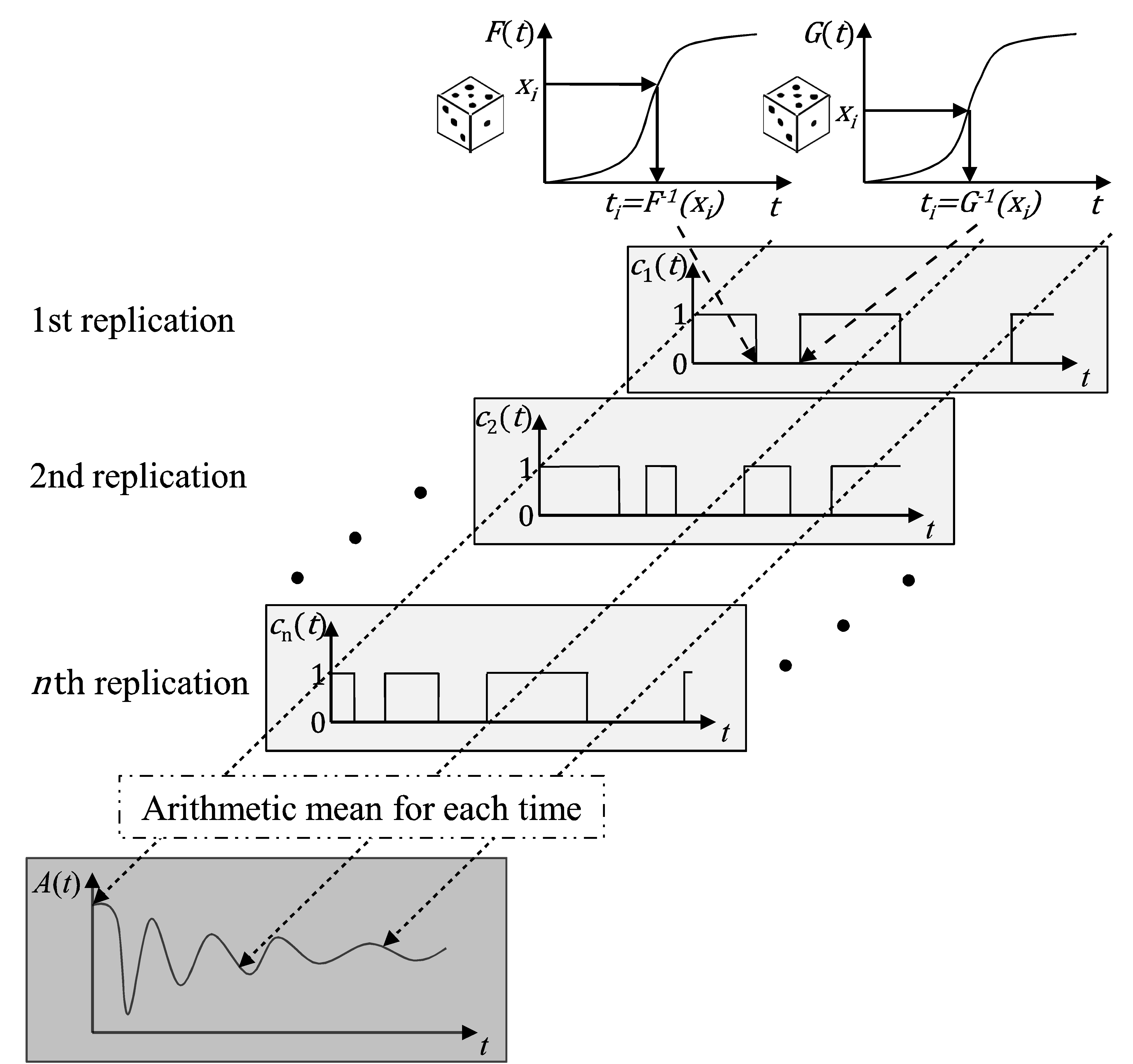Figure 2. Monte Carlo simulation of (point-) availability [20].

Firstly, random failure and repair times are generated based on the given cdfs of failure and repair behavior. Correspondingly, pseudorandom numbers within the bounds 0 and 1 are generated. These random numbers are interpreted as the failure  or repair  probabilities. The failure and repair times  can subsequently be determined based on these random failure and repair probabilities and using the inversion method [21]:

By alternatively selecting one of the randomly generated failure and repair times , one trajectory of the state indicator is established. As for the renewal process, the starting condition  is assumed: The component is thus starting in a new condition at time .

After establishing one state indicator throughout the entire observation time, the procedure is repeated  times.  is given as the number of Monte Carlo replications. As a result,  trajectories of the state indicator are calculated. Finally, the time-dependent availability  can be derived as the arithmetic mean of all generated state indicators for each time.

It should be mentioned that the calculated availability represents an approximate solution. The statistical quality of the values determined by means of the Monte Carlo simulation can be estimated. According to the central limit theorem [21], (17) is valid for the random number  according to (18) [22].

This means that the estimated random number normally follows an asymptotic distribution, with the expected value  and the variance . Based on this thesis, the statistical quality of the mean value determined with the help of the Monte Carlo simulation can be specified as a level of statistical quality.

4.       Confidence Intervals

Selected fundamentals for determining confidence levels are presented in this chapter. After the basic definition, the bootstrap method is presented in greater detail.

4.1.  Basic Definition of Confidence Level

The confidence level  of availability  can be determined in an analogous manner to the reliability [23]. According to (19), it can be calculated using the integral of the density with the considered value  as a lower limit:

The calculation is based on the density  of the availability. The confidence level describes the fact that a minimum availability value  is reached with a probability of . One inherent part of a certain confidence level is the specification of the probability . As a sample, the 95% confidence level implies that the observed value is at least the certain value  in 95 out of 100 cases. Usually, a confidence interval lies symmetrically to the median. This means that a 90% confidence interval is bounded by the 5% and 95% confidence level.

There are several methods for determining the confidence intervals of a distribution function. Table 2 shows the most commonly used methods, which can be divided into “analytical methods”, “approximate methods” and “simulation-based methods”. The table itself is based on [24].

An analytical description of the availability function is required in order to determine a confidence interval with analytical or approximate methods. However, if general scenarios are considered or the Monte Carlo simulation is used, this analytical description is not present or modelled implicitly into an algorithm. Even in the case that the analytical formulation is absent, the bootstrap methods are suitable for determining confidence levels of availability. However, the confidence level determined by bootstrapping is also an approximate solution.

Table 2. Most commonly used methods for determining a confidence interval.

Analytical methods	Approximate methods	Simulation-based methods
·   Beta-binomial distribution ·   Likelihood ratio Interval ·   Bayes confidence interval	·   Fisher matrix ·   Wald method ·   Wilson score interval	·   Bootstrapping: Non-parametric bootstrapping Parametric boot­strapping

4.2.  Bootstrapping

Bootstrapping [25] is a method of resampling and suitable for statistical evaluation, especially if the parameters of a given sample cannot be determined using other analytical methods [26]. The method was first introduced by Bradley Efron [27]. There are two different types of bootstrapping according to Figure 3: non-parametric and parametric bootstrapping.

Non-parametric bootstrapping starts with a given sample
with sample size . First, a bootstrap sample  is established by drawing  random numbers from  with replacement and without regard to the order. Afterwards, using well-known standard parameter estimators such as the Maximum Likelihood Method (MLE) [13], the parameters  of the bootstrap sample are estimated so that the cdf obtained by bootstrapping , named as realization, can be identified.

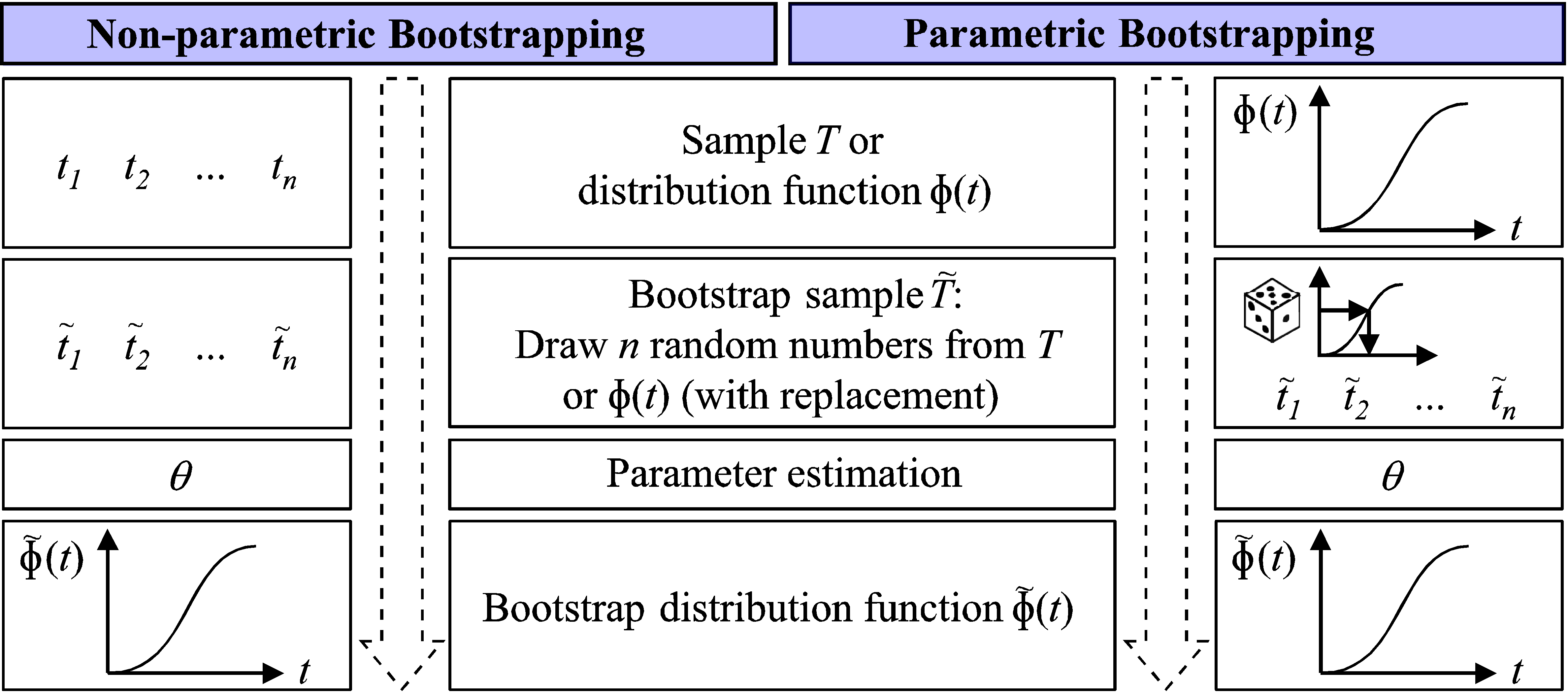Figure 3. Non-parametric (left) and parametric (right) bootstrapping [28].

In contrast to non-parametric bootstrapping, the parametric bootstrap method is based on a given distribution function . If this cdf is not given in advance, it can be estimated using well-known estimators such as the MLE or by employing the non-parametric bootstrap method. The first step of parametric bootstrapping is to generate  random failure times from the given distribution function. This is performed in the same manner as for the Monte Carlo simulation: with the help of pseudorandom numbers and the inversion method. The distribution function by means of bootstrapping  will subsequently be determined in the same manner as non-parametric bootstrapping, i.e., using standard parameter estimators.

Several bootstrap confidence intervals are available for analyzing the confidence level by bootstrapping [2]. The evaluation can be carried out as [29]:

• An empirical bootstrap confidence interval
• A standard bootstrap confidence interval
• A percentile bootstrap confidence interval
• A bootstrap-t-confidence interval
• A BCα confidence interval

Irrespective of the type of bootstrap confidence level, the bootstrap method needs to be carried out  (number of bootstrap replications) times. As a consequence,  realizations of the distribution function ,  can be identified. This array of trajectories subsequently has to be evaluated. Figure 4 shows the procedure for determining a confidence level using the bootstrap method.

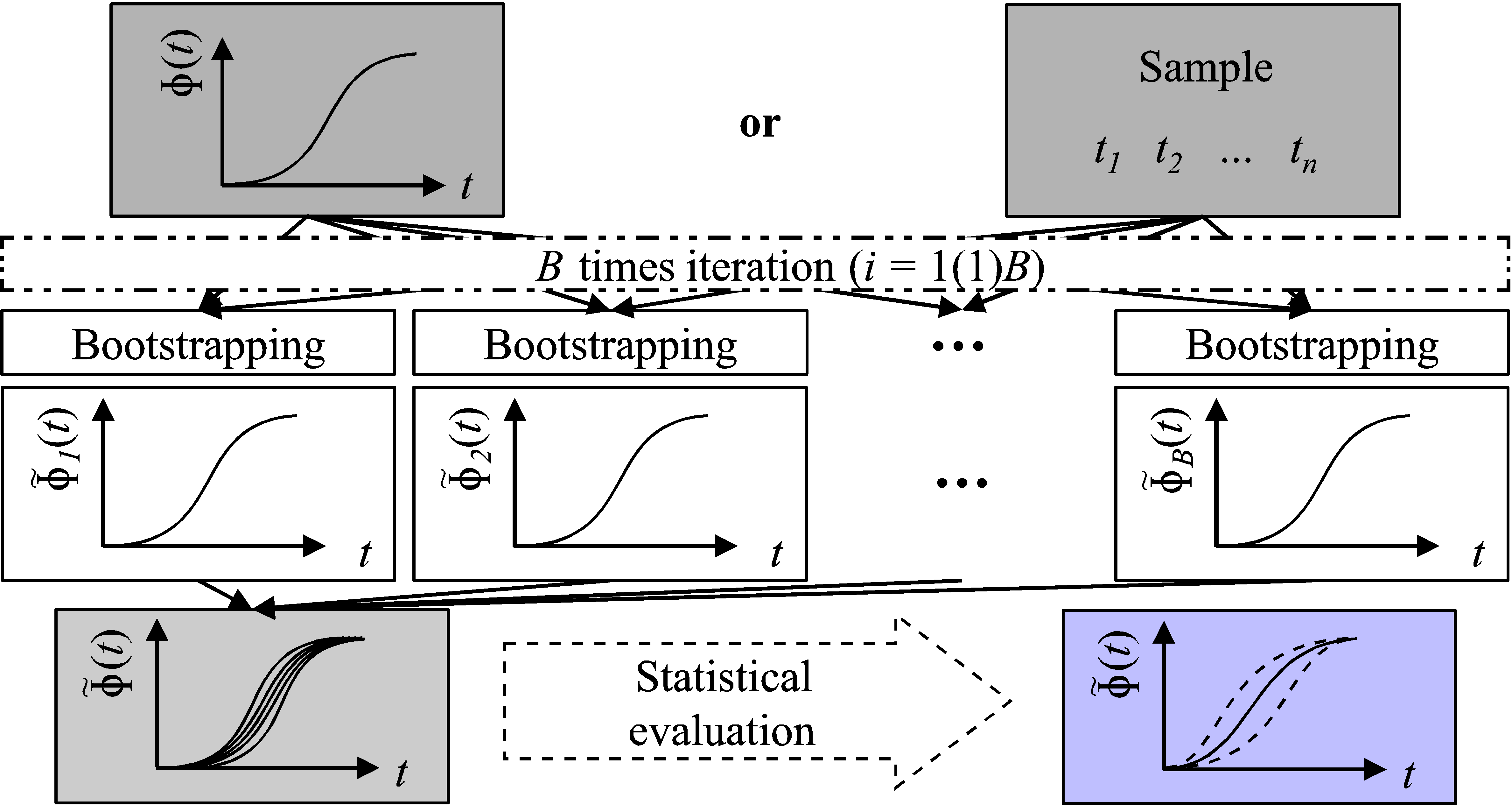Figure 4. Determining a confidence level using bootstrapping.

In the following, only the “empirical bootstrap confidence interval”, the “standard bootstrap confidence interval” and the “percentile bootstrap confidence interval” are presented in greater detail. If an empirical bootstrap confidence interval is calculated, the trajectories are evaluated by performing an empirical bootstrap density function  for each time . Based on the percentiles of these density functions, the confidence level of the original distribution function can be determined.

It is likewise possible to calculate a “standard bootstrap confidence interval”. Under the assumption that the realizations  are roughly normally distributed, the upper and lower confidence limit of the 100(1‑2α)% standard bootstrap confidence interval can be calculated for each time  as:

 is the arithmetic mean value of the  realizations , where  is given as the standard deviation of these realizations.  is the αth quantile of the standard normal distribution.

On the other hand, the percentile bootstrap confidence interval can be selected based on the given  realizations . They have to be sorted in ascending order. Consequently, the  is the ith smallest element. Afterwards, the 100(1‑2α)% percentile bootstrap confidence interval can be determined according to (21). Here,  equals the largest integer less than or equal to .

In general, the input parameters of the bootstrap parameter can be variously interpreted as failure or repair times. As an example, the given cdf  can either be a failure or a repair distribution function. The confidence interval calculated using the bootstrap method can thus be the confidence interval for a failure distribution function or a repair distribution function. The confidence level of a reliability function or other distribution functions using the bootstrap method is calculated in the same way.

5.       Bootstrap Monte Carlo Simulation

This section presents the bootstrap Monte Carlo simulation as a new method for availability inference and demonstration with a confidence level. Using this highlighted method, the confidence level of point-availability as well as the confidence level of average and steady-state availability can be determined.

5.1.  Basic Concept

The bootstrap Monte Carlo simulation (BMCS) combines bootstrapping as a method for determining confidence levels with the Monte Carlo simulation. Figure 5 shows the basic principle of BMCS for calculating point-availability with a confidence level. With this basic principle, it is possible to use the information concerning the confidence level of the input data, i.e., of the failure and repair distributions.

The BMCS can be carried out based on pure samples or on the distribution functions (cdfs) of failure and repair behavior. It is also possible to shuffle both types of input data, such as by providing the failure behavior as a cdf and the repair behavior as a sample of repair times or vice versa. The basic procedure also facilitates individual sample sizes for lifetime and repair data. In other words, the sample sizes do not have to be equal.

In the first step of the BMCS, one realization  of the failure behavior and one realization  of the repair behavior are generated using the bootstrap method and based on the input data. Depending on the type of input data, non-parametric or parametric bootstrapping is employed. After this, these realizations are used to calculate one realization of the point-availability  using the Monte Carlo simulation, according to Figure 2. After repeating the entire calculation  times,  realizations of point-availability ,  can be calculated.  corresponds to the predefined number of bootstrap replications. Finally, this array of trajectories of point-availability subsequently has to be evaluated.

As shown in the previous chapter, it is possible to determine an empirical bootstrap confidence interval, a standard bootstrap confidence interval, a percentile bootstrap confidence interval or another type of bootstrap confidence interval. If an empirical bootstrap confidence interval is chosen, an empirical bootstrap probability density function  is derived from the individual function values of the realizations of point-availability.

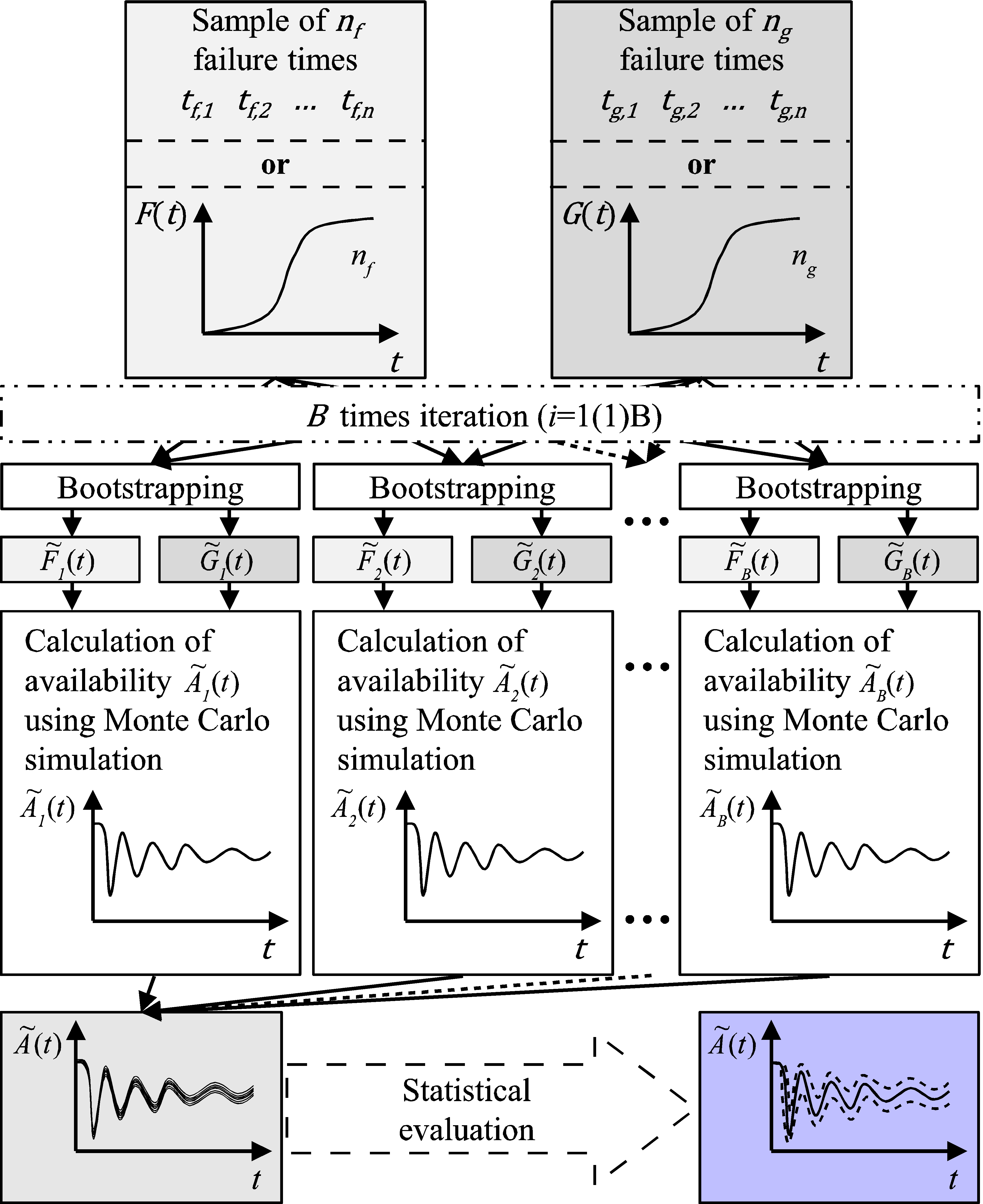Figure 5. Basic procedure of bootstrap Monte Carlo simulation (BMCS) for calculating point-availability with a confidence level.

The confidence interval can be derived based on the percentiles of these density functions. Figure 6 illustrates this step of the statistical evaluation. On the other hand, the standard bootstrap confidence interval can be determined according to (20) or the percentile bootstrap confidence interval according to (21).

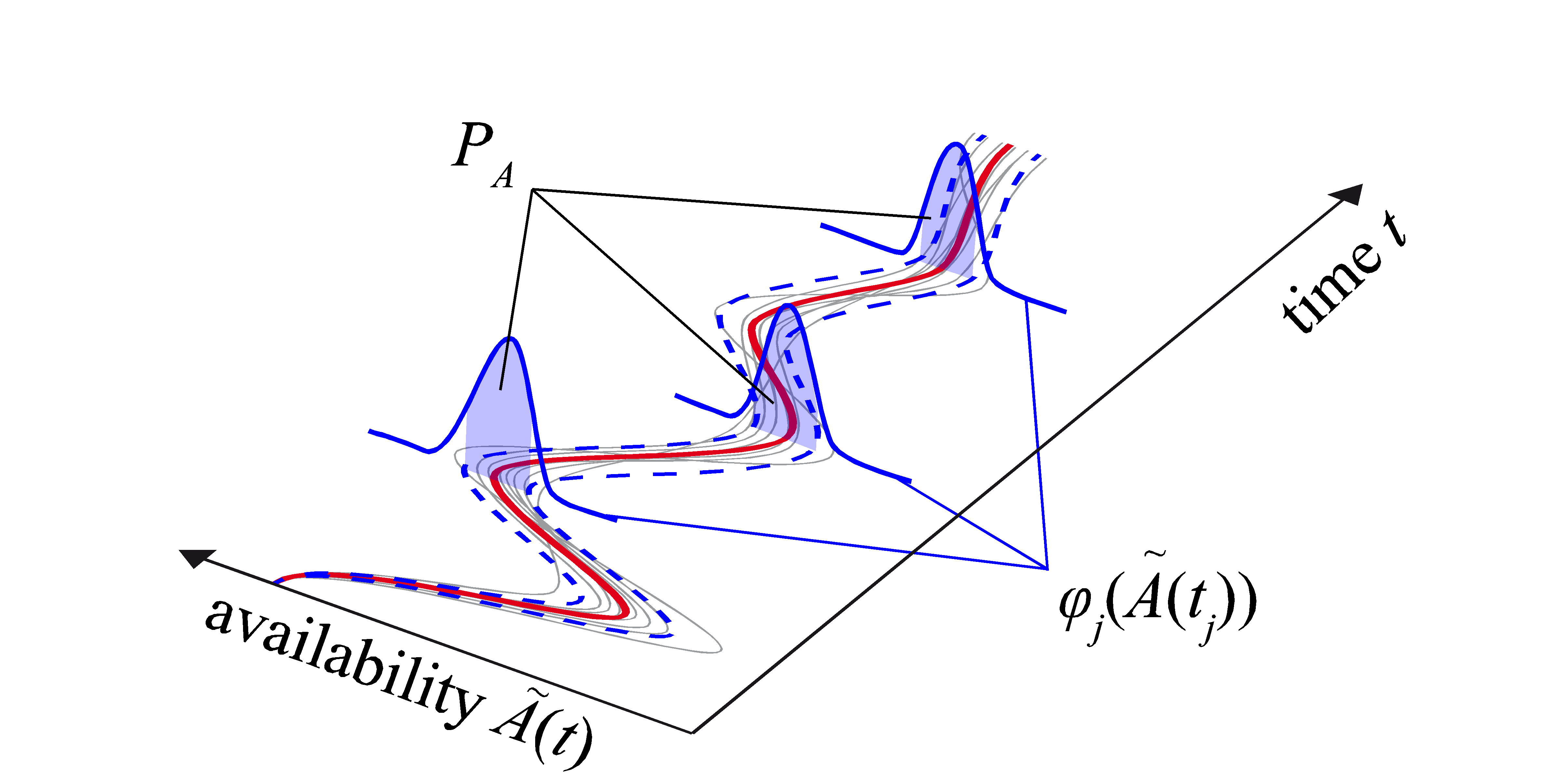Figure 6. Statistical evaluation of the realizations of point-availability.

The BMCS is an approximation method as the Monte Carlo simulation is used: The calculated confidence interval is thus also an approximation. The BMCS can only provide accurate approximations from a certain threshold number of replications. As shown in [28], the number of bootstrap replications should not be fewer than 200. If at least 200 bootstrap replications are carried out, the approximation of the BMCS is very thorough. On the other hand, the number of Monte Carlo replications should be chosen in the range of 1,000-10,000 Monte Carlo replications. Generally speaking: The higher the numbers of replications, the better the approximation of BMCS. It should be mentioned that the simulation time increases sharply in line with higher numbers of replications.

If the Markov process is used in place of the Monte Carlo simulation to calculate point-availability within the basic procedure according to Figure 5, the bootstrap Markov process (BMP) is established (see [1] or [6], for example). The BMP combines the bootstrap method with the calculation of availability using the Markov method. The BMP therefore has the same restrictions as the Markov process. In other words, the failure and repair behavior needs to be exponentially distributed.

Besides the BMCS and the BMP, the bootstrap renewal process (BRP) [6] combines the bootstrap method with the renewal process [1]. In other words, the availability calculation of the basic procedure according to Figure 5 is carried out using the alternating renewal process. All three methods – the BMCS, the BMP and the BRP – facilitate the availability prediction and demonstration with confidence level, whereby the BMCS has the highest potential to be extended to more general scenarios of availability prediction and demonstration.

5.2.  Steady-State and Average Availability with Confidence Level

It is likewise possible to estimate a confidence interval for steady-state and average availability using the bootstrap Monte Carlo simulation provided in Figure 5. The basic concept needs to be amended so that steady-state or average availability is determined for each bootstrap replication  with , as opposed to point-availability. The calculation of steady-state availability is performed using (7), whereas the average availability is calculated according to (8). In total,  realizations of the value of steady-state availability  or  realizations of the curve of average availability  are generated.

Exactly as with point-availability, both the  realizations of steady-state availability and the  realizations of average availability are evaluated statistically. An empirical, standard or percentile bootstrap confidence interval can thus be constructed.

5.3.  Sample Calculation

In the following section, a sample calculation using the BMCS is presented. The sample calculations determine point-availability, steady-state availability and average availability with a confidence level. The availability values are calculated with a 90% confidence interval for the sample failure and repair behavior listed in Table 3.

Table 3. Sample failure and repair behavior.

Failure behavior	Repair behavior
·   Weibull-distributed · · · ·	·  Sample ( ) of repair times [h]:
	154.0 171.5 183.0 193.0 201.5	209.5 217.0 224.0 231.0 239.0	246.0 254.0 262.0 271.0 280.5	291.5 304.0 320.0 342.5 382.0

The failure behavior  is given as a cdf, whereby the repair behavior  is based on a given sample. As shown in Table 3, the sample sizes of the failure and repair behavior are not equal. The BMCS is carried out with 200 bootstrap and 10,000 Monte Carlo replications. Within the last step of the BMCS, an empirical bootstrap confidence interval is determined.

To begin with, Figure 7 shows the  realizations of the point-availability calculated during the BMCS. Furthermore, the mean availability and the 90% confidence interval of the time-dependent availability are illustrated. Some empirical density functions  of the confidence interval are also plotted on the graph. The color of the pointed density functions clarifies the frequency . In other words, this color illustrates the number of availability curves going through the point  in absolute terms.

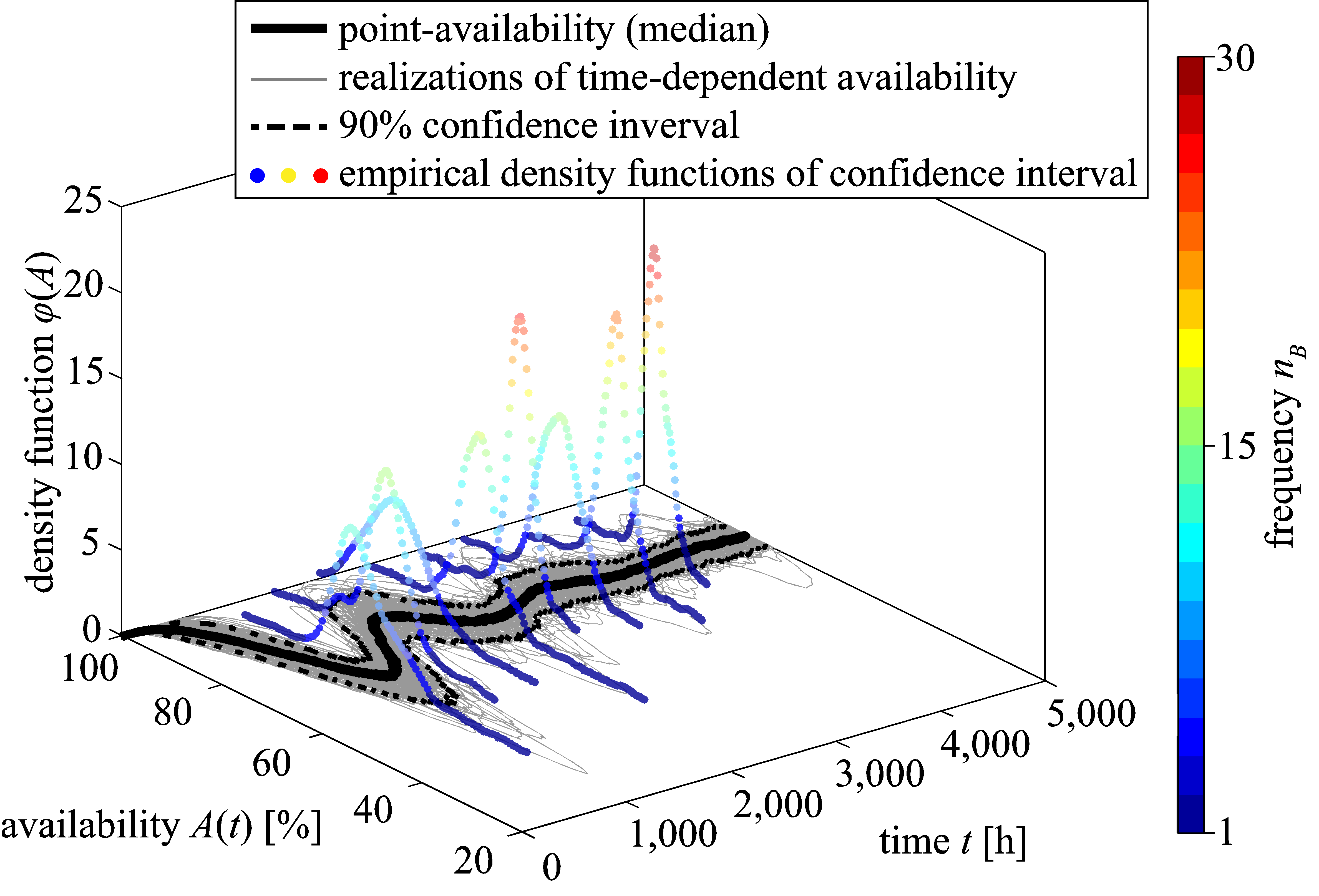Figure 7. Point-availability with 90% confidence interval and selected density functions of confidence level.

Figure 8 builds on Figure 7 to show the steady-state availability as well as the average availability. Both availability graphs are clarified with a 90% confidence interval. The confidence interval of all graphs expands slightly with shorter durations and converges to a constant range at longer ones. For long operation times, the confidence intervals of all types of availability coincide with each other and lead to a constantly wide range.

Although it is not necessary to carry out this investigation because non-parametric bootstrapping is applied to the sample of the repair behavior, the analysis of the repair times using the Maximum Likelihood method provides a lognormally distributed repair behavior ( , , ).

As shown in [1] and [6], the confidence interval of all types of availability becomes narrower or smaller as the sample sizes increase. Independently of the sample sizes, the confidence interval of point-availability, steady-state availability and average availability harmonizes very well within a constantly wide range for long operation times. A first verification of the BMCS as well as an investigation about the accuracy of the BMCS is provided by Müller et al. [30]. If the numbers of bootstrap and Monte Carlo replications are high enough, the BMCS provides acceptable results as an approximate method. First parameter studies of the input parameters of the BMCS are carried out in [1], [20] or [30].

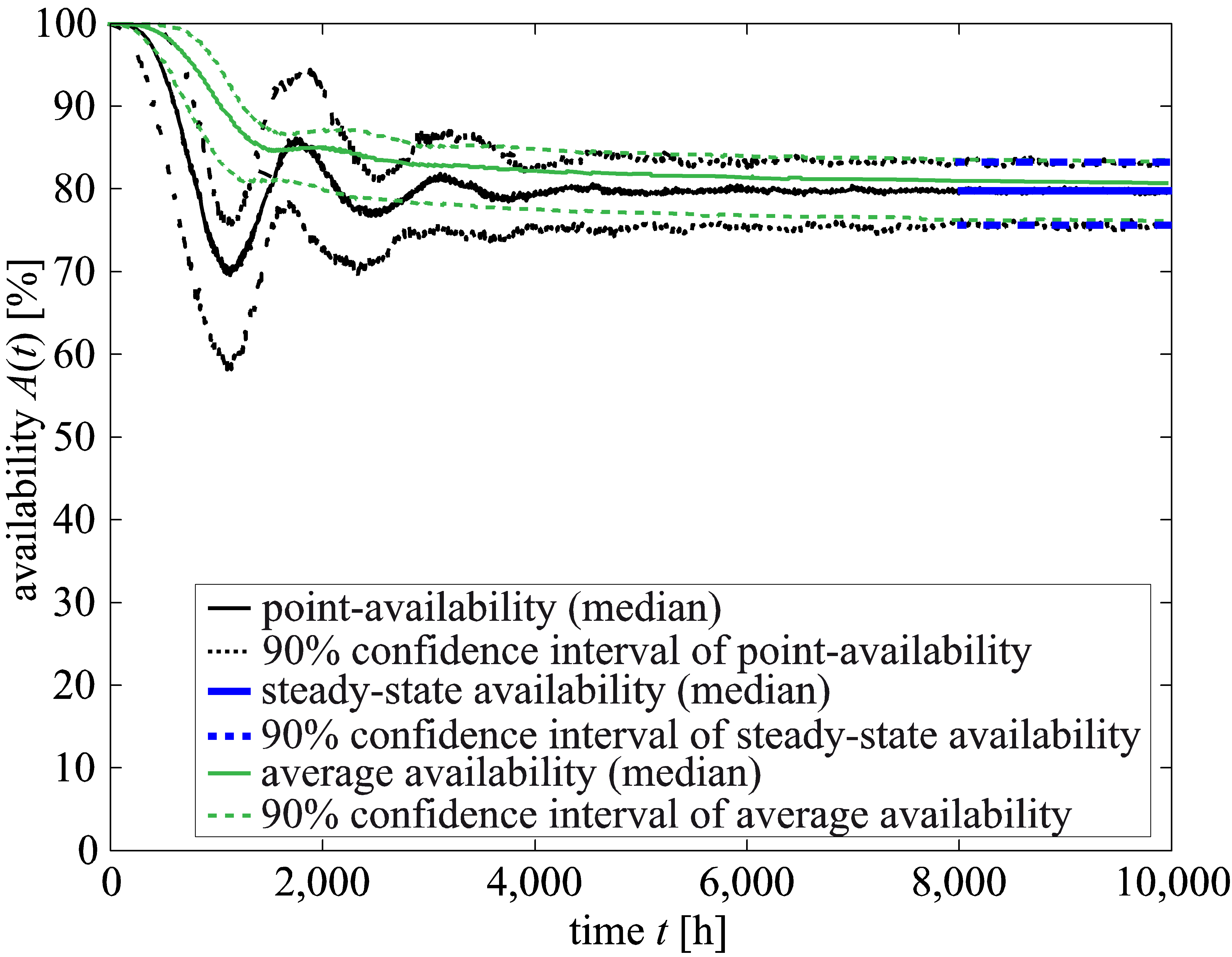Figure 8. Point-availability, steady-state availability and average availability with 90% confidence interval.

6.       Availability Demonstration Test with Consideration of Confidence Level

In this section, the inverse bootstrap Monte Carlo simulation (IBMCS) as a new procedure is presented. The IBMCS enables an availability demonstration test with consideration of confidence levels to be conducted. Firstly, the basic concept of IBMCS is presented in detail before a sample calculation is carried out.

6.1.  Inverse Bootstrap Monte Carlo Simulation

An availability demonstration test needs to be carried out in order to demonstrate the quality of a repairable system. This test provides the demonstration that the system will operate with a stated level of availability. As a consequence of the availability description with confidence level using the BMCS, the availability demonstration tests also need to be specified with a confidence level. The inverse bootstrap Monte Carlo simulation (IBMCS) enables such availability demonstration tests with consideration of confidence levels. The new procedures provide a test plan comprising the required number of failures that must be observed to demonstrate a certain availability value  at a specific point in time . The IMBCS can be seen as the inversion of the BMCS. Figure 9 shows the basic concept of the inverse bootstrap Monte Carlo simulation.

The procedure begins by defining the input data. The objective is to determine the required number of observed failure and repair times, i.e., the required sample size  and  of failure and repair behavior to demonstrate the availability value  at time  with confidence level . It is assumed that the failure behavior  and repair behavior  of the repairable system or product is known, but not its corresponding sample sizes. Furthermore, the ratio of sample sizes of failure and repair behavior is predefined:

Besides the ratio of the sample sizes, the minimum  and maximum number of observed failure time  are also predefined. These numbers correspond with the minimum and maximum number of reliability tests that could be carried out. Frequently, the maximum number of possible tests is fixed by other limitations, e.g., the number of available test benches. The minimum number is usually fixed by the corporate strategy or normative rules. These requirements frequently require a certain minimum number of reliability tests to be carried out.

Finally, the calculation parameters  (number of bootstrap replications of the BMCS) and  (number of Monte Carlo replications of the BMCS) are required.

In the first step of the IBMCS, a BMCS is carried out based on the input data. In other words, an availability value  with confidence level  is calculated using the BMCS and under the assumption of the minimum sample size of failure behavior . The same calculation is carried out under the assumption of the maximum sample size , so that the availability value  with confidence level  can be determined.

It should be noted that the corresponding sample size of the repair behavior can be calculated for each step of the IBMCS using the predefined value of ratio  according to (22) using the actual sample size of failure behavior.

After determining both values  and , it must be verified whether the objective availability value  lies within these ranges. In other words, a check is conducted as to whether (22) is valid or not.

There is no solution if (22) is not valid, since the objective availability value does not lie within the interval of possible availability values ]. Values which are not included in this interval cannot be achieved with the predefined limitations of minimum and maximum failure time figures.

If the calculation can be advanced further, as (22) is valid, a binary search is performed to determine the required number of observed failure and repair times. Therefore, in the first step, a new sample size number is chosen according to (23), where
and .

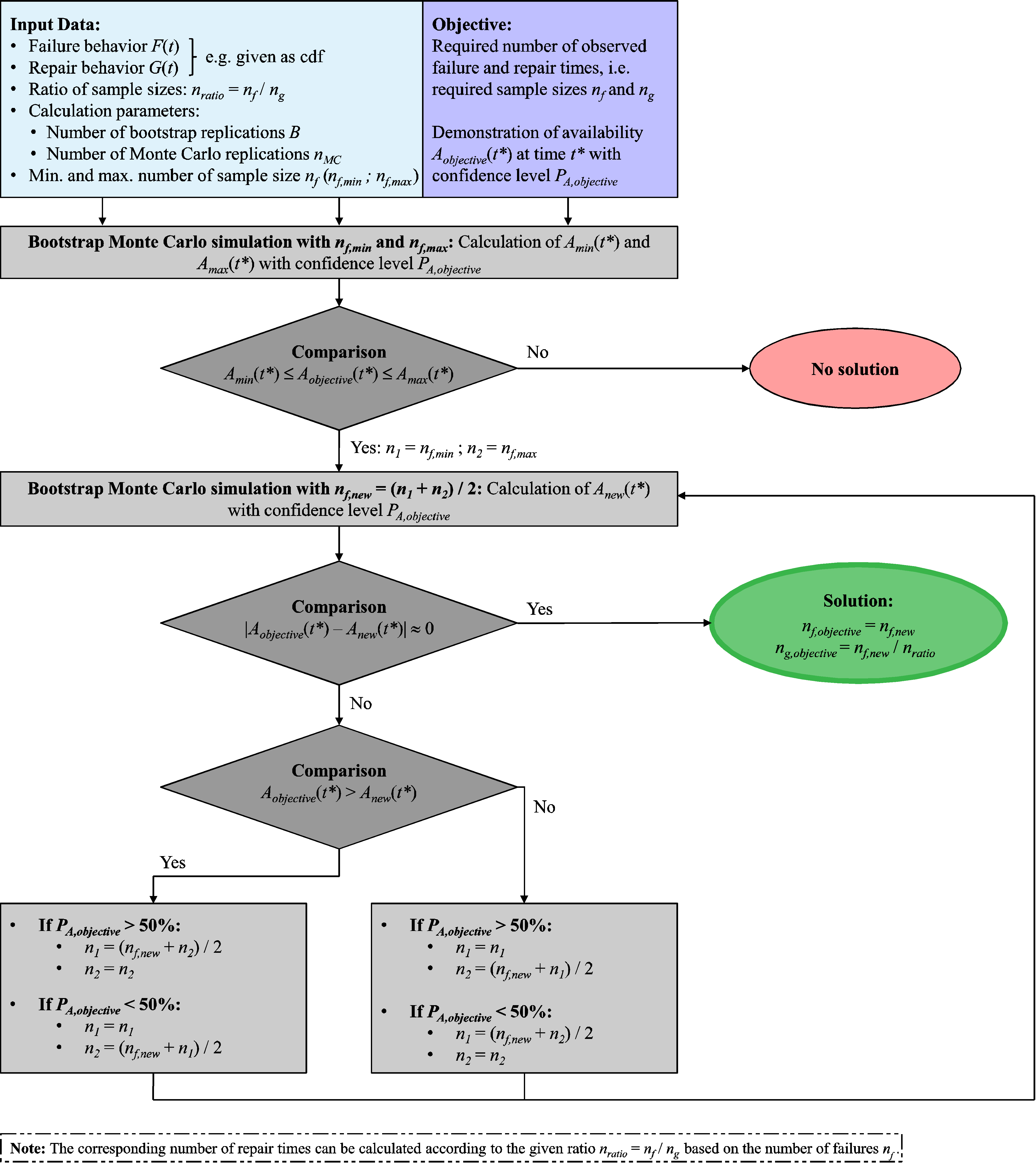Figure 9. Basic procedure of the inverse bootstrap Monte Carlo simulation (IBMCS).

The new value  is derived as the mean of the previous sample sizes due to the binary search. After this, a new calculation using the BMCS gives the availability value  with confidence level  based on the new sample size . If this value is not approximately equal to the required demanded availability value , the sample size requires further adaptations. Therefore, two case distinctions have to be made. One distinction investigates if the objective availability value  with confidence level  is greater than the actual calculated availability value  with confidence level .

Furthermore, the second distinction has to be made with regard to the demanded confidence level . As shown in Figure 10, the availability value with a constant confidence level increases in line with increasing sample sizes if the confidence level is lower than 50%. On the other hand, if , the availability value decreases as sample size  increases.

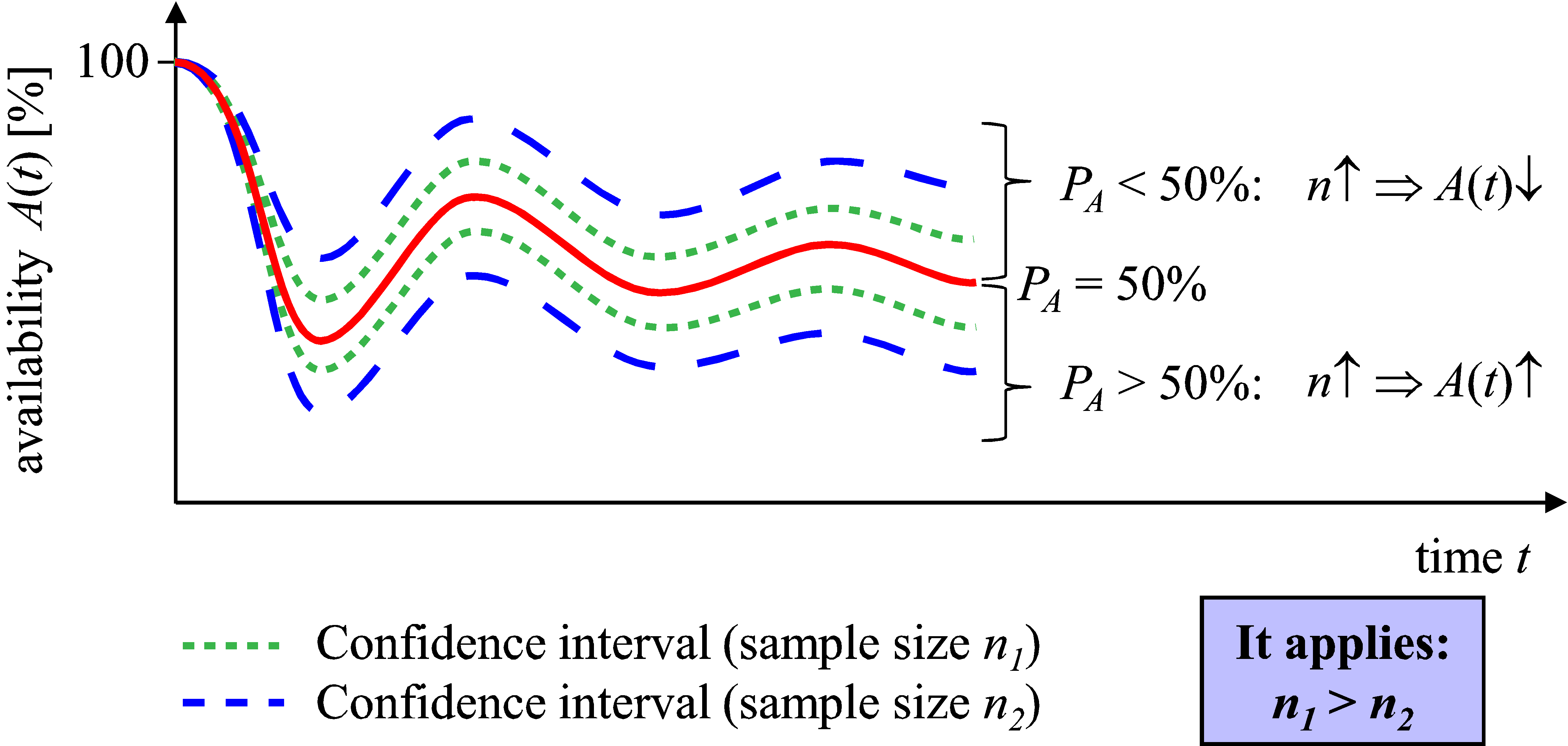Figure 10. Confidence intervals with varying sample sizes.

After performing both case distinctions, the sample size of the failure behavior is adapted according to the equations shown in Figure 9. The corresponding number of observed repair times is calculated according to (22). A new availability value  with confidence level  based on the new sample sizes is subsequently determined using the BMCS.

These calculation steps are repeated until the actual determined availability value  with confidence level  and corresponding sample sizes   and  is approximatively equal to the objective availability value  with confidence level . If this is the case, the required number of failures and repair actions that must be observed in order to demonstrate a certain availability value is determined as:

As a derivation of the IBMCS, it is possible to conduct an availability demonstration test with consideration of the confidence level. It is therefore possible to demonstrate a specific availability value for a point in time and a given confidence level. The procedure yields the required number of failures as well as the required number of repair actions that must be observed within a reliability test of the investigated repairable system or product with a known failure and repair behavior type. The availability test plan can subsequently be conducted and several availability requirements can be demonstrated with a confidence level.

The IBMCS can be adapted further so that it is not the value of point availability  at time with confidence level  is demanded within the objective, but rather the value of average availability  at time with confidence level . In this case, the point-availability value is not calculated, but rather the average availability value within the inherent steps of BMCS. The IBMCS procedure is carried out in the same manner.

If the BMP or BRP is used within the basic procedure according to Figure 9 as opposed to the BMCS, the inverse bootstrap Markov process (IBMP) or the inverse BRP (IBRP) are established.

6.2.  Sample Calculation

In the following section, a sample calculation of the IBMCS is presented. The procedure is applied to the system already investigated in the previous sample calculation. In other words, the failure behavior of the system is given from previous investigations as being Weibull-distributed with ,
and . The repair behavior is given as being lognormally distributed with ,
and .

The IBMCS is carried out with 200 bootstrap replications and 10,000 Monte Carlo replications. It is assumed that an availability of 75% should be present at an operating time of 5,000 h. The availability should be indicated with a confidence level of 95%. It is possible to carry out a maximum of 100 reliability tests. In other words, the maximum number of sample sizes for the failure behavior is 100. The ratio between both sample sizes is predefined as 2, i.e., the sample size of the repair behavior should be half of the sample size of the failure behavior.

On the basis of the IBMCS, it is possible to determine the required sample size of failure behavior to  and the sample size of the repair behavior . Assuming that the failure behavior is known and constant as given, 16 failures need to be observed during the reliability test in order to demonstrate the demanded availability of 75% with a 95% confidence level at a time of 5,000 h. In other words, the analysis of the given failure behavior must be based on 16 failure times. Conversely, the analysis of the repair behavior must simultaneously be based on 8 observed repair times.

Figure 11 shows point-availability with a 90% confidence interval. The confidence interval is determined with input data from  and . As illustrated in this figure, the requirements of 75% availability with a 95% confidence level at an operating time of 5,000 h can be demonstrated with the given sample sizes.

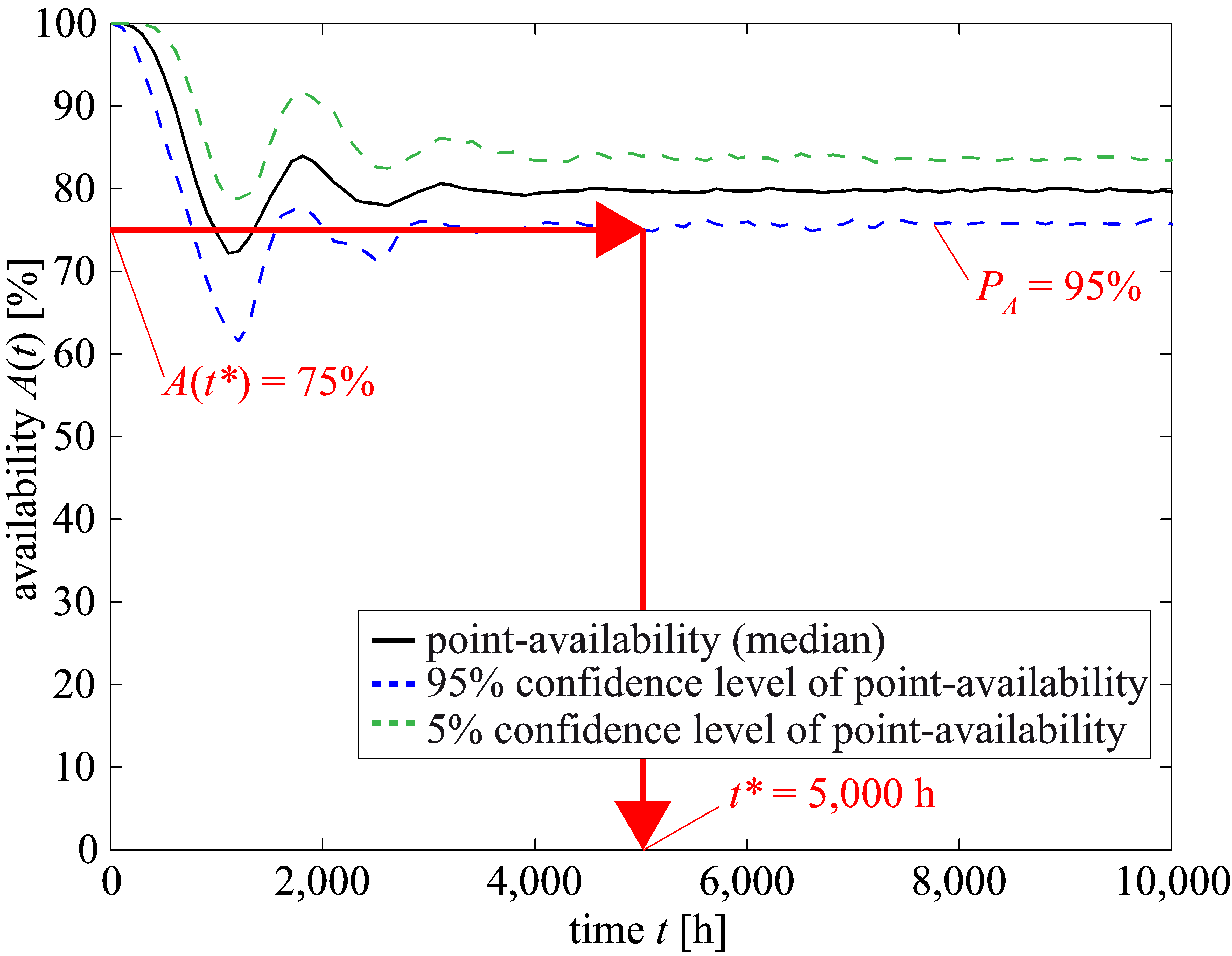Figure 11. Point-availability with 90% confidence interval based on 16 failure and 8 repair times.

7.       Potential of the Bootstrap Monte Carlo Simulation and the Inverse Bootstrap Monte Carlo Simulation

Both the bootstrap Monte Carlo simulation (BMCS) and the inverse bootstrap Monte Carlo simulation (IBMCS) have a high potential to be applied to more general availability scenarios. Beyond the consideration of preventive maintenance, the BMCS and the IBMCS are not restricted to selected maintenance strategies. It is possible to investigate technical systems with general maintenance strategies.

As given in [31], different maintenance strategies are conceivable. In general, the maintenance strategy defines the type and planning of the intended maintenance activities [31]. Possible strategies include corrective, preventive or condition-based maintenance actions. Furthermore, combined strategies are possible. Besides the aspect of maintenance, the BMCS and IMBCS have a high potential to take system aspects, failure dependencies or limited maintenance resources into consideration.

The BMCS and the IBMCS are very innovative in terms of the possibility of applying them to more general scenarios. This also includes transferring the procedures to predict and demonstrate reliability with a confidence level, e.g., for systems with periodical maintenance (see [28] or [30]).

8.       Summary & Conclusions

In this paper, the bootstrap Monte Carlo simulation (BMCS) is highlighted as a new method for availability inference and demonstration with a confidence level. Besides the BMCS, the bootstrap Markov process (BMP) and the bootstrap renewal process (BRP) are briefly outlined. The BMCS facilitates analysis based on a sample of failure and repair times or on a mean value distribution with corresponding sample sizes of failure and repair behavior. The BMCS has no restrictions concerning the distribution function.

The inverse bootstrap Monte Carlo simulation (IBMCS) is presented in detail alongside the BMCS. The IBMCS enables the planning of availability demonstration tests with consideration of confidence levels. The procedure is based on the BMCS. Using the IBMCS, it is possible to determine the required number of failures and repair actions that must be observed in order to demonstrate a certain state of availability with a predefined confidence level.

Firstly, the fundamentals of reliability engineering and a basic definition of repairable systems and availability were given. After this, the bootstrap method for determining a confidence level of a distribution function was shown in more detail. After describing the BMCS in detail, a sample availability calculation with a confidence level was carried out. Based on the BMCS, the IBMCS was derived. The basic procedure was outlined on the basis of a sample calculation, too. Finally, the potential of the BMCS and the IBMCS was investigated.

The BMCS and the IBMCS have high potential for application to more general scenarios concerning general systems. Besides corrective maintenance actions, other maintenance strategies can be included within the procedure. Both the BMCS and the IBMCS are very innovative. In addition to availability with a confidence level, further parameters of reliability engineering, e.g., reliability, can be integrated into the BMCS and IBMCS.

Conflict of Interest

The authors declare that there are no conflicts of interest.

1. F. Müller, P. Zeiler, B. Bertsche, “Availability Demonstration with Confidence Level Based on Reliability and Maintainability” in Proc. of Annual Reliability and Maintainability Symposium (RAMS 2017), Orlando, USA, 2017.
2. C.E. Ebeling, An Introduction to Reliability and Maintainability Engineering, Mc Graw-Hill: New York, 1997.
3. A. Krolo, B. Bertsche, “An Approach for the Advanced Planning of a Reliability Demonstration Test based on a Bayes Procedure”, in Proc. of Annual Reliability and Maintainability Symposium (RAMS 2003), Tampa, USA, 2003.
4. J.-H. Lim, S.W. Shin, D.K. Kim, D.H. Park, “Bootstrap Confidence Intervals for Steady-State Availability” in Asia-Pacific Journal of Operational Research, Vol. 21, No. 3, 2004, pp. 407-419.
5. J.-C. Ke, Y.-K. Chu, “Nonparametric Analysis on System Availability: Confidence Bound and Power Function” in Journal of Mathematics and Statistics, Vol. 3, No. 4, 2007, pp. 181-187.
6. P. Zeiler, F. Müller, B. Bertsche, “New methods for the availability prediction with confidence level” in Proc. of European Safety and Reliability Conference (ESREL 2016), Glasgow, Scotland, 2016.
7. A. Coppola, “Some observations on demonstrating availability” in RAC Journal (the Journal of the Reliability Analysis Center), Vol. 6, No. 1, 1998, pp. 17-18.
8. W. Wang, D.B. Kececioglu, “Confidence Limits on the inherent availability of equipment” in Proc. of Annual Reliability and Maintainability Symposium (RAMS 2000), Los Angeles, USA, 2000.
9. V.P. Singh, S. Swaminathan, “Sample Sizes for System Availability”, in Proc. of Annual Reliability and Maintainability Symposium (RAMS 2002), Seattle, USA, 2002.
10. J.S. Usher, G.D. Taylor, “Availability Demonstration Testing” in Quality and Reliability Engineering International, Vol. 22, 2006, pp. 473-479.
11. B. Le, J. Andrews, C. Fecarotti, “A Petri net model for railway bridge maintenance” in Proc. of the Institution of Mechanical Engineering Part O: Journal of Risk and Reliability, Vol. 231(3), 2017, pp. 306-323.
12. G.A. Pérez Castañeda, J.-F. Aubry, N. Brinzei, “Stochastic hybrid automata model for dynamic reliability assessment” in Proc. of the Institution of Mechanical Engineering Part O: Journal of Risk and Reliability, Vol. 225(1), 2011, pp. 28-41.
13. B. Bertsche, Reliability in Automotive and Mechanical Engineering, Springer: Berlin, Heidelberg, 2009.
14. F. Beichelt, Reliability and Maintenance. Networks and Systems, CRC Press: Boca Raton, 2012.
15. F. Beichelt, Applied Probability and Stochastic Processes, CRC Press: Boca Raton, 2016.
16. A. Fritz, “Berechnung und Monte-Carlo Simulation der Zuverlässigkeit und Verfügbarkeit technischer Systeme (Calculation and Monte Carlo simulation of reliability and availability of technical systems)”, PhD Thesis, University of Stuttgart, 2001.
17. A. Fritz, P. Pozsgai, B. Bertsche, “Notes on the Analytic Description and Numerical Calculation of the Time Dependent Availability” in M. Nukulin, N. Limnios (eds), Proc. International Conference on Mathematical Methods in Reliability (MMR 2000), Bordeaux, France, 2000, pp. 413-416.
18. R.Y. Rubinstein, D.P. Kroese, Simulation and the Monte Carlo Method, John Wiley & Sons, Inc.: New Jersey, 2008.
19. E. Zio, The Monte Carlo Simulation Method for System Reliability and Risk Analysis, Springer: London, 2013.
20. F. Müller, “Integration der Aussagewahrscheinlichkeit in die Berechnung und Simulation der Verfügbarkeit (Integration of the Confidence Level in the Calculation and Simulation of Availability)”, Master Thesis, University of Stuttgart, 2015.
21. VDI-Guideline 4008-6, Monte-Carlo-Simulation, VDI: Düsseldorf, 1999.
22. P. Poszgai, “Realitätsnahe Modellierung und Analyse der operative Zuverlässigkeitskennwerte technischer Systeme (Close-to-Reality Modelling and Analysis of the Operational Reliability Characteristics of Technical Systems)“, PhD Thesis, University of Stuttgart, 2006.
23. P. Zeiler, B. Bertsche, “Component reliability allocation and demonstration test planning based on system reliability confidence limit” in Proc. European Safety and Reliability Conference (ESREL 2015), Wroclaw, Poland, 2015.
24. G. Yang, Life Cycle Reliability Engineering. John Wiley & Sons, Inc.: Hoboken, New Jersey, 2007.
25. B. Efron, R.J. Tibshirani, An Introduction to the Bootstrap. Champ & Hall / CRC: Baca Raton, London, New York, Washington, 1993.
26. C.E. Lunneborg, Data Analysis by Resampling: Concepts and Applications, South Western, USA, 2000.
27. B. Efron, “Bootstrap Methods: Another Look at the Jackknife” in The Annals of Statistics, Vol. 7, No.8, 1979, pp. 1-26.
28. F. Müller, P. Zeiler, B. Bertsche, “Bootstrap-Monte-Carlo-Simulation von Zuverlässigkeit und Aussagewahrscheinlichkeit bei periodischer Instandhaltung (Bootstrap Monte Carlo Simulation of Reliability with Confidence Level regarding Periodical Maintenance)” in 28. VDI-Fachtagung Technische Zuverlässigkeit 2017, Entwicklung und Betrieb zuverlässiger Produkte, VDI-Berichte 2307, VDI: Düsseldorf, 2017, pp. 69-81.
29. W.Q. Meeker, L.A. Escobar, Statistical Methods for Reliability Data. John Wiley & Sons, Inc.: New York, Chichester, Weinheim, Brisbane, Singapore, Toronto, 1998.
30. F. Müller, P. Zeiler, B. Bertsche, “Bootstrap Monte Carlo Simulation of Reliability and Confidence Level with Periodical Maintenance” in Forschung im Ingenieurwesen, 2017, DOI 10.1007/s10010-017-0220-6, pp. 1-11 (online first article).
31. P. Zeiler, B. Bertsche, “Availability modelling and analysis of an offshore wind turbine using Extended Coloured Stochastic Petri Nets” in Proc. of European Safety and Reliability Conference (ESREL 2014), Wroclaw, Poland, 2014.

(Click to view)

(Click to view)