1. Introduction

Recently, we reported a system having as a purpose the calculation of the sun trajectory during one day in a specific location [1]. In this paper, another system presenting enhanced capabilities with respect to the system presented in the above work is reported.

The energy that can be extracted from a flat solar collector depends to a large extent on the direction of solar radiation in relation to the surface of the panel. This will be maximum, when the sun rays and the surface are perpendicular to each other. Through, a solar tracking system the above condition can be fulfilled the whole time. However, it is cheaper and simpler to keep a fix solar collector for a period of time than to make two rotations along two different axes to achieve tracking. In systems with dual axis tracking the panel is rotated along the line pointing to the vertical of the place (surface azimuth angle) and it is rotated along the line east-west (tilt angle or slope).

In general, for the fixed panels the optimal surface azimuth angle is zero degrees. Therefore, the tilt angle is the only one that is adjusted to maximize the collected energy. In this respect, several studies to obtain the optimum tilt angle  at different locations of the world have been conducted. As for example: Athens [2], Izmir [3], four places in India [4], 5 regions in China [5], Sanliurfa [6], Tabass [7], two locations in India [8], eight provinces of Turkey [9], New Delhi [10], Helwan [11], Brunei [12], Syria [13], Surabaya [14], 35 sites of the Mediterranean region [15], Taiwan [16], Madinah [17] and the examples could continue.

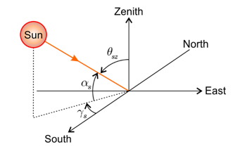Figure 1. Sun position relative to one fixed point on Earth.

In the literature, it is suggested that in the northern hemisphere the panels must be facing south. The optimum tilt angle depends of the geographical latitude of the place . Not all of the studies are focusing in the calculation of an annual . In some cases, this angle is reported in monthly or biannual (twice a year) time periods. Because, the selection of different time periods impacts the efficiency of the solar collector. For example, it was reported that in Madinah, a monthly adjustment of the tilt angle can enhance in 8% the captured energy than the one that can be obtained when this angle is kept fix during the whole year [17]. Numerous suggestions for  are found in the literature. For example, in the References [3, 11, 18] is proposed , in the Reference [19] is suggested , where the minus sign refers to the summer season and the plus sign is for the winter. In the Reference [10] is proposed  for the winter and  for the summer. In the Reference [20] is recommended , in the Reference [21] is suggested , in the Reference [22] is proposed , where  is the declination and the examples could continue. Unfortunately, the only way to obtain the optimum tilt angle is through radiation measurements at the place of interest for an extended period of time. This is due to the fact that solar radiation has different components, which are the direct, the

diffuse and the albedo radiation. The optimum tilt angle, which is the ones that maximize the energy extraction is influenced in the way that these radiation components are distributed.

In this work, a system for estimation of the tilt angle considering exclusively the direct radiation is presented. This can be used in the locations that does not have a record of radiation measurements, or when the users or designers of the solar installations do not have a direct access to available radiation data. With this system in a very few minutes and with a minimum of interaction of the end user, several data used in the solar designs are obtained. Also, the tilt angle is calculated in time periods of six minutes, daily, monthly, biannual and yearly. A comparison of the energetic gain when the tilt angle changes at the different time periods is made as well. Finally, a comparison was made between the results provided with the proposed system and the ones reported for the monthly tilt angle of 22 different places. The root mean square error ( ) obtained through this comparison was between 1.5 and 9.5 degrees. The estimation of the monthly tilt angle deviated in average for less than 6.3°. Also, an adjustment for each of the estimated monthly slope angles is proposed, which might reduce the energy loss.

2.       Direct Radiation Incident on a Tilted Solar Flat Panel

2.1.  Sun Position

In a fixed point on the Earth, due to the Earth’s rotation and its movement around the sun, the direction of the beam radiation is changing in time. It is customary to describe the trajectory that follows the sun by using two angles, when the representation of the Celestial sphere is used. These are: the hour angle  and the declination angle for an equatorial coordinate system and the solar altitude angle  and the solar azimuth angle  for a horizontal coordinate system. The angle between the two planes; the one containing the Earth’s axis and the meridian plane of the point of observation, and the other containing the Earth’s axis and the meridian plane of the sun is . At solar noon, i.e., when the sun is on the observer meridian . The angle between the equator and the sun position at solar noon is the declination. This angle in degrees is given by [23]

where  is the integer day number, being January 1st . The declination is changing in time, but during one day is almost constant.

      In the Figure 1 are shown the angles ,  and , where the latter angle is the solar zenith angle.  is the angle between the direct sun rays and the horizontal plane of the specific location,  when the sun is on the horizontal plane,  when the sun is at the zenith. During the sun hours this is an angle between  and  . Its value is negative before sunrise and after sunset. The relationship between the solar altitude angle and solar zenith angle is .  is the angle between the south and the projection of the direct sun rays on the horizontal plane. This is an angle between  and . Displacements east of the south are negative and west of the south are positive.

In the References [24-28] have been reported algorithms to calculate the sun position. The complexity and accuracy differ from each other. In this work, the fifth algorithm of the Reference [28] is employed, because it is easier to program and it is accurate from 2010 to 2110. The output of this algorithm are the angles , ,  and . The inputs are the date (month, day, year), the time in decimal format, the latitude, the local longitude  , the atmospheric pressure  and the room temperature . In this algorithm, the following conventions are applied: the latitude is an angle between  and , in locations up north of the equator it is positive, otherwise is negative. The longitude is an angle between  and , being  at the prime meridian. At the east of this meridian has a value between  and . It is measured in a counter clockwise fashion to the east.

The angles of the equatorial and horizontal coordinate systems are related to each other by [18]

and

where the sign function is equal to  , if  is positive; otherwise is .

2.2.  Angle of Incidence on a Tilted Flat Solar Collector

In a fixed location, the sun moves across the sky along the day. By this reason, the beam radiation vector will make an angle  with respect to the normal of the collector surface. Most solar energy can be captured when . If a unit vector  is pointing from a fixed point in the Earth to the direction of the beam radiation and another unit vector  is normal to the collector surface, the angle between both vectors can be computed with the dot product, i.e., .

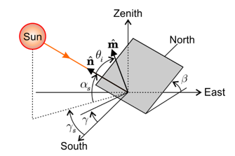Figure 2. Flat surface rotated along the lines east-west and south-north.

To minimize the angle  during a specific time period, the fixed flat solar panels are subjected to two rotations. On one hand, the panel is rotated in a counterclockwise fashion an angle  along the line east-west (tilt angle or slope). On the other hand, the panel is rotated in a clockwise fashion an angle  along the line pointing to the zenith of the place (surface azimuth angle). Both rotations are shown in the Figure 2.

According to the geometry shown in the Figure 2. The unit vectors  and  are given by

Thus, the angle of incidence between both vectors after a few simplifications is

The tilt angle is an angle between  and , when  the collector is facing the south, which is the most used slope in the northern hemisphere. If the panel is horizontal  and . Finally, if the surface of the panel is facing the north. In most situations, the collectors are adjusted to have an azimuth angle . This angle is varied, when there are objects that produce shadows over the collector surface, or in some cases when a set of two fixed panels are used for extracting energy. In this configuration, one of them is used in the morning and the other is employed after the solar noon [14].

2.3.  Maximization of the Flux of Energy in Terms of the Tilt Angle

Recently, Handoyo and co-workers have exposed a mathematical procedure to calculate the optimum tilt angle of a solar flat collector [14]. In that work,  is expressed in the equatorial coordinate system in terms of the following angles: , , ,  and . This equation is reported elsewhere as in Reference [18]. They do the first derivative and the second derivative test for a single variable to maximize  in terms of . At first,  is calculated and later the condition  is tested. These tests will be applied to , which is expressed in terms of a horizontal coordinate system. The value of , which corresponds to the critical point of is

Computing  of requires as inputs the date (month, day and year), the hour in decimal format, the geographical coordinates and the panel azimuth angle. If the magnitude of any of these variables changes, the value of  is modified as well.

2.4.  Sunrise, Sunset, Day Length and Local Standard Time

In the equator, the day length is 12.0 h during the whole year. But at latitudes different to this geographical point, this quantity is changing in daily basis. Up north of this latitude, during the summer the sun light is shining for a longer time, on the contrary during the winter. Therefore, the net energy that can be captured by a collector will depend to some extent on the day length. Of course, if there is no sun light, no solar energy can be obtained. By this reason, it is interesting to calculate the evolution of this variable, which is related to the sunrise and the sunset time. From , the sunrise hour angle in degrees can be obtained by making , i.e.,

      The sunset hour angle is . The day length  in decimal hour is

The solar time  in decimal hour is related to the hour angle by

In terms of the local standard time  and a time correction factor  is

The time correction factor in minutes is given by

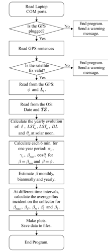Figure 3. Flowchart of the Python program.

where  is the standard longitude,  is the observer’s longitude,  is a time correction due to the daylight-saving time (DST) and  is the equation of time. In the following conventions must be employed:  is an angle between  and . It is considered negative at the west of the Greenwich meridian, and positive at the east of it. In this work, the DST changes are not considered, thus . Also, , where  is the time zone in decimal hour.  is positive at the west of the prime meridian and negative at the east of it.

      By combining and , it can be obtained the local standard time in decimal hour as                                .

With and the sunrise time  is obtained. Similarly, by substituting  in (16) the sunset time  is obtained.

The coordinated universal time   is employed to calculate the sun position. It is related to the  by                                   .

This time doesn’t observe the DST, and   follows the same convention applied to .

3.       System Description

3.1.  GPS Receiver

The global positioning system (GPS) receiver used in this work was the model ND-105C GPS Dongle from GlobalSat WorldCom Corporation. But, any GPS receiver that meets the National Marine Electronics Association (NMEA) requirements and that has the possibility of sending sentences through the serial port can be employed.

The above GPS receiver for the output data follows the protocol NMEA 0183. It returns four the sentences: GGA, GSA, GSV and RMC. The GGA sentence contains all the useful data introduced as an input in the program as the validity of satellite fix, the geographical latitude with the corresponding hemisphere and the local longitude with its relative position with respect to the prime meridian.

3.2.  Python Program

The program used to perform the calculations was written in Python 3.6. It can be requested by email to the corresponding author. The flowchart of the program is shown in the Figure 3.

The time frame set in the calculations corresponds to one year. They will begin in the first day of the month at which the program was run, and they will end in the same day and in the same month of the next year.

The Spyder integrated development environment (IDE) included in the Anaconda distribution was chosen to debug and to run the program. The communication between the GPS and the computer is realized through the serial port. Therefore, pyserial module must be installed, it is freely available at: (https://pypi.python.org/pypi/pyserial). In order to the program to work properly the end user must provide the communication (COM) port at which the GPS is connected to the computer and it must configure the time zone of the Windows operating system (OS). This must correspond to the region at which the calculation of the tilt angle is going to be done. The DST changes are not considered in the program, and they must be ignored in the above configuration.

      As it shown in the Figure 3, if the GPS is plugged, the GPS sentences are read through the serial port. From the GGA sentence all the required inputs are extracted (valid fix,  and ). When the fix is invalid the program will stop displaying a warning message. Otherwise, the program will continue doing computations. From the OS the date and the  are read by the program.

To obtain  the program computes and . The first equation requires the declination, which is calculated with . The latitude is provided by the GPS.  is obtained with , when  is substituted by  , which is obtained with .  is get when  is substituted by  in . The zenith angle at solar noon is calculated with the declination and the latitude. For places with greater latitudes than the tropics, this angle never will reach zero. For both tropics will be zero once a year. In places between the above latitudes will be reach zero twice a year.

Once the daily behavior of  and  are obtained a daily time interval is set for the calculation of the variables , ,  and . Initially, is evaluated with two different tilt angles (  and ). A few averages are realized once  is obtained. These are done for the following time periods: daily  , monthly , from April to September and from October to March (biannual)  and yearly .

However, the magnitude of the above angles depend of the daily time interval selected in the simulation. For example, their magnitude will have one value for the daily time interval  h, which differs to the obtained if  h is considered. Therefore, a daily time interval for the simulation must be chosen. In this work, the user can select one of two possible options for the daily time interval. The first comprehends the daily time interval  in steps of 0.1 h (six minutes). The initial time of this interval is , and the final time of this interval is . This daily time interval will be called long time. The functions  and  are referring at the maximum and minimum values that reaches the variable over a one year period. The second time interval will be called short time. This is the default time considered in the program. It is given by  in steps of 0.1 h. It is worth mentioning, that the user can input the magnitude of , which appears in the coefficient  of , but its default value is set to . If  is chosen in the simulations, for some days and in some specific times could result that .This means that the sun is not in the local horizon. In these particular situations, the program assign NaN values to all variables.

To estimate the average flux of solar radiation incident in the solar collector, the different values of  ( , , ,  and ) are evaluated in (6). Finally, the average of  for the each of the above angles in different time periods is calculated.

All the calculated variables are saved in files, which have a comma separated value (csv) format. The plots of the yearly evolution of , , ,  at the solar noon, , and  are generated by the program. In addition, the plot of the annual variation of  is generated, when is evaluated with the following angles: , , ,  and . After this step, the program ends.

3.3.  System Applications

The applications that can have the system can be briefly summarized as follows:

• To have an insight of the working hours of the solar installations during a whole year, because these can operate just during the sun hours. The above variable is related to the day length, the sunrise and sunset times, which are provided graphically and in csv format files.
• To control a dual axis tracking system by the knowledge of the solar azimuth and the solar altitude angles. Both angles are provided by the system.
• To estimate the tilt angle that should follow one single axis tracking system in different periods of time. This can be done every six minutes, daily, monthly or biannual. To have an insight of the energetic gain that can have any of the above systems.
• To modify the program to extend its capabilities.

4.       Results and Discussion

As stated above, the system can work at different locations. Just two conditions must be meet. On one hand, the correct COM port at which the GPS is detected by the computer must be set. On the other hand, the time zone of the location and the configured in the OS must match.

Several tests were realized to verify the proper operation of the system. However, they were realized in different places of same city, which was Mexico City.

As an example of the output data provided by the program, the results obtained during one test made in Mexico City will be presented.

4.1.  Annual Evolution of , ,   and  at Solar Noon

In the Figure 4 the plot of  for 366 days is shown. The minimum value of the sunrise time is 6:09 h and it will be reached in June 6th, 2017. The maximum value is 7:17 h and it will be reached in January 19th, 2018. Due to the geographical location of Mexico City, there is no a significant daily variation associated to this variable.

In the Figure 5 is shown the plot of the yearly variation of . The minimum value of the sunset time is 17:52 h and it will occur in November 23rd, 2017. The maximum value is 19:14 h and it will occur in July 6th, 2017.

In the figure 6 the yearly evolution of  is presented. The shortest day length will be in December 21st, 2017 and it has a value of 10 h and 49 min. It is not surprising that this date corresponds to the winter solstice. The day length reaches a maximum value of 13 h and 10 min. This will happen in June 21th, 2017, which corresponds to the summer solstice.

In the Figure 7 the yearly evolution of the  at solar noon is presented. Due to the fact that Mexico City is located between the equator and the Tropic of Cancer, twice a year  is zero at solar noon. One of these dates corresponded to May 18th, 2017 and the other will occur in July 25th, 2017. The global maximum of  is  and it will be reached in the winter solstice. The local maximum, with a value of 3.94°, will happen in June 21st, 2017, which corresponds to the summer solstice.

Once  and  are known the daily time interval (  or ) is obtained.

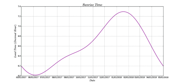Figure 4. Yearly evolution of the sunrise time

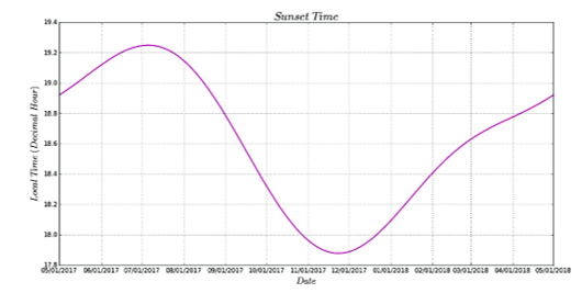Figure 5. Yearly evolution of the sunset time.

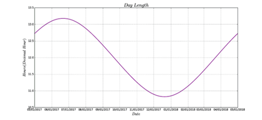Figure 6. Yearly evolution of the day length.

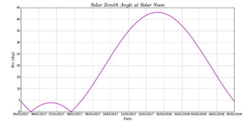Figure 7. Yearly evolution of the solar zenith angle at solar noon.

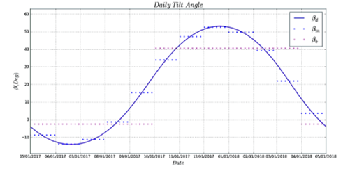Figure 8. Yearly evolution of the daily, the monthly and the biannual tilt angles.

4.2.  Estimation of the Tilt Angle

In the Figure 8 are shown the values of ,  and , which were obtained averaging . This angle was calculated in steps of 0.1 h. The simulation was made by choosing the daily time interval as .As it can be seen in the figure 8 from April 23th to August 18th the daily tilt angle must be negative. It means that during this period the solar collector must face to the north. When a monthly adjustment of the tilt angle is realized, the panel should face the north from May to August. As well as  from April to September. In the Figure 9 it is shown how  is varying during an entire year in terms of the angles , , , and , where .

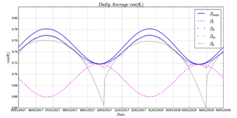Figure 9. Yearly evolution of average radiation flux incident on the collector surface. When different tilt angles are evaluated in (6).

Table 1. Report summarizing the generated results of the program.

Time Period	(Deg)						(h)	(h)	(h)
May, 2017	−8.73	0.763	0.753	0.752	0.752	0.679	12.93	6.09	19.01
June, 2017	−13.7	0.779	0.768	0.768	0.76	0.661	13.16	6.04	19.19
July, 207	−11.22	0.77	0.76	0.759	0.756	0.67	13.05	6.17	19.22
August, 2017	−1.18	0.742	0.736	0.735	0.734	0.698	12.64	6.35	18.99
September, 2017	15.41	0.721	0.72	0.718	0.681	0.717	12.09	6.47	18.56
October, 2017	33.98	0.73	0.727	0.725	0.717	0.708	11.53	6.6	18.13
November, 2017	47.23	0.761	0.751	0.75	0.749	0.68	11.06	6.84	17.9
December, 2017	52.61	0.779	0.768	0.768	0.758	0.662	10.84	7.13	17.97
January, 2018	49.76	0.768	0.758	0.757	0.753	0.672	10.97	7.28	18.25
February, 2018	39.29	0.739	0.733	0.731	0.73	0.699	11.36	7.17	18.52
March, 2018	22.06	0.72	0.719	0.717	0.678	0.716	11.89	6.82	18.7
April, 2018	3.68	0.733	0.729	0.727	0.72	0.707	12.45	6.39	18.84
Yearly	19	0.751	0.743	0.742	0.732	0.689	12	6.61	18.61
April-September	−2.48	0.755	0.748	0.747	0.738	0.693	12.72	6.25	18.97
October-March	40.6	0.753	0.747	0.745	0.735	0.694	11.27	6.97	18.24

As expected, the greater flux incident on the collector surface is obtained when the panel is moved every six minutes. Surprisingly,  doesn’t vary much when is evaluated with ,  or . In September and in March a biannual movement of the panel can provide less energy than the energy extracted with the tilt angle equal to the latitude of the location. Most of the year,  will have the smallest magnitude.

One file with the csv format summarizing the above results is generated, when the program is executed. This report is presented in the Table 1

The Table 1 must be read in the following way. The first twelve rows are referred to the monthly values. Taking as an example the month of May,  should be , the radiation flux incident on the collector surface in average will be 0.763, 0.753, 0.752, 0.752, 0.679, when  is evaluated in with angles , , , and , respectively. The day length will be 12.93 h in the decimal hour, and the sunrise and the sunset times will be 6.09 h and 19.01 h, respectively. Both values are as well given in decimal hour.

It is not very surprising to find that the yearly tilt angle is almost equal to the latitude as it is shown in the first column of the table 1, that is . In the last two rows of the first column the results for  are shown. As expected yearly  is 12.0 h. Finally, in the row related with the yearly values, and average of  for the different tilt angles is shown. These magnitudes are 0.751, 0.743, 0.742, 0.732 and 0.689, for , , , and , respectively. It is interesting to note that an energetic gain of ~1% is obtained by adjusting the tilt angle every six minutes than doing it every month.

4.3.  Evaluation of the Algorithm

The optimum tilt angle at a given location requires of the measurements of the solar radiation. Therefore, to evaluate the algorithm one comparison was made between the results obtained and the results reported for the monthly tilt angle of 22 different places. To do this comparison the geographical coordinates were input manually to the algorithm. The monthly optimum tilt angle of this places is reported in the References [3-13]. As a measure of the deviation the  was calculated. This is given by

where  and  are two time series, and  in is the number of data. The results of this comparison are shown in the Table 2. During these simulations the daily time interval was always .            In each of the rows corresponding to the twelve months of the year the difference between the reported tilt angle and the calculated with the algorithm is shown. A negative sign means that  was underestimated, on the contrary the angle was overestimated. In these simulations, the average  always was overestimated as it can be seen in the last row. Near the winter and summer solstices the variation was larger than in other months. The better estimations of  were obtained in March and in October. The greatest was found for the city of Mohe (9.21°). The smallest discrepancy for this variable was found for the city of Aligarh (1.59°).

Table 2. Comparison between the results of this work and the results of 22 locations reported in the literature.

City	Jan. (Deg)	Feb. (Deg)	March (Deg)	April (Deg)	May (Deg)	June (Deg)	July (Deg)	Aug. (Deg)	Sept. (Deg)	Oct. (Deg)	Nov. (Deg)	Dec. (Deg)	RMSE (Deg)
Izmir	0	−1	−1.5	1.6	6.9	8.6	9.7	3.8	-0.2	−1.7	-0.5	0.6	4.46
Sanya	6.07	6.16	3.84	−0.24	-0.44	−0.57	-1.36	−0.22	1.79	4.75	6.13	8.31	4.32
Shanghai	10.54	6.52	6.6	5.77	5.69	5.54	6.17	4.86	4.39	6.53	10.26	9.13	7.10
Zhengzhou	9.42	6.58	4.95	5.36	6.94	8.02	7.73	6.14	6.21	6.87	6.42	8.18	7.00
Harbin	3.11	1.41	2.12	7.36	11.32	14.87	13.4	9.5	4.03	2.12	3.19	4.48	7.85
Mohe	0.57	−2.71	-0.64	6.9	15.53	17.47	16.56	11.05	4.09	1.09	0.65	1.62	9.21
Lhasa	−0.1	-0.02	0.1	1.37	4.87	6.61	5.45	3.35	0.4	−0.98	-0.9	0.59	3.06
Sanliurfa	5.31	3.47	−1.5	−4.31	−5.87	−5.81	−5.48	−4.05	−1.53	3.32	4.59	5.98	4.52
Tabass	−0.65	−1.63	−1.97	0.77	5.98	3	5.35	2.9	−2.23	−2.86	−1.34	0.07	2.94
Aligarh	1.09	−0.07	−0.87	1.08	1.12	−3.94	−1.6	2.15	−0.82	−1.1	0.25	1.26	1.59
Adana	5.94	4.05	2.95	3.99	7.36	6.41	8.75	5.23	2.87	1.88	4.23	6.62	5.39
Ankara	7.1	5.38	3.82	6.46	9.1	10.21	10.55	5.85	3	2.42	5.47	8.78	7.01
Diyarbakır	5.47	3.66	1.86	4.22	7.72	7.8	10.14	4.53	0.9	−0.39	2.81	6.16	5.44
Erzurum	2.25	1.49	1.83	6.34	8.9	10.01	10.35	5.69	2.94	1.51	2.64	3.96	5.79
Istanbul	8.91	7.23	5.8	6.58	8.28	11.42	10.75	7.01	3.05	4.34	7.32	10.6	7.99
Izmir	5.12	4.3	2.52	4.9	7.4	8.5	9.86	5.25	1.62	1.34	3.54	6.85	5.70
Samsun	7.52	6.85	6.41	7.17	9.87	12	11.33	6.58	4.63	4.92	5.89	8.19	7.93
Trabzon	8.34	7.67	8.24	9.01	9.71	11.84	11.16	9.42	7.45	6.75	7.73	9.02	8.97
New Delhi	1.4	2.28	−0.75	0.2	2.12	−2.94	−0.6	3.11	−0.91	1.69	1.55	2.06	1.85
Helwan	7.37	0.26	−0.62	−5.46	−0.45	−5.47	−6.11	−9.41	−6.06	−5.17	2.58	6.05	5.37
Darussalam	9.86	7.24	3.92	−5.4	−5.55	−5.63	−3.31	−5.6	−1.22	10.73	7.69	8.55	6.75
Damascus	0.79	−0.49	−0.86	2.17	6.54	8.76	7.7	3.65	−0.59	−1.5	−0.07	1.07	4.10
Average tilt angle deviation ( )	5.02	3.11	2.1	2.99	5.59	5.75	6.2	3.67	1.53	2.11	3.64	5.36

      In each of the rows corresponding to the twelve months of the year the difference between the reported tilt angle and the calculated with the algorithm is shown. A negative sign means that  was underestimated, on the contrary the angle was overestimated. In these simulations, the average  always was overestimated as it can be seen in the last row. Near the winter and summer solstices the variation was larger than in other months. The better estimations of  were obtained in March and in October. The greatest was found for the city of Mohe (9.21°). The smallest discrepancy for this variable was found for the city of Aligarh (1.59°).

4.4.  Correction Factor

The results of the section 4.3 suggests that by considering exclusively the direct sun radiation,  is overestimated. Therefore, we propose an empirical expression, in which the monthly tilt angle might be estimated better by

where  is a new estimation of the monthly tilt angle and  is the correction factor, which can be obtained from the last row of the table 2. This correction might help to improve the value of the monthly tilt angle calculated with the program presented in this work.

5.       Conclusions

A system for the estimation of the tilt angle in different world locations has been implemented. The computation of this angle is realized for different time periods.

Data provided by a GPS receiver are automatically passed to an algorithm without the intervention of the user. This approach might be more effective and it may avoid errors.

The code is written in a high-level programming language, which makes the process of increasing its capabilities simpler.

The estimation of the yearly evolution of average radiation flux incident on the collector surface for different angles shows that the monthly variation of the tilt angle produces almost the same energetic gain than moving this angle every six minutes.

Conflict of Interest

The authors declare no conflict of interest.

Acknowledgment

The authors want to thank to the Instituto Politécnico Nacional (IPN) and the Comisión de Operación y Fomento de Actividades Académicas COFAA-IPN for the financial support provided to do this work.

1. J. Fonseca-Campos, L. Fonseca-Ruiz, P. N. Cortez-Herrera “Portable system for the calculation of the sun position based on a laptop, a GPS and Python” in 2016 IEEE International Autumn Meeting on Power, Electronics and Computing (ROPEC 2016), Ixtapa Mexico, 2016. https://doi.org/10.1109/ROPEC.2016.7830580
2. E. D. Mehleri, P. L. Zervas, H. Sarimveis, J.A. Palyvos, N. C. Markatos, “Determination of the optimal tilt angle and orientation for solar photovoltaic arrays” Renew. Energ., 35(11), 2468–2475, 2010. https://doi.org/10.1016/j.renene.2010.03.006
3. H. Gunerhan, A. Hepbasli, “Determination of the optimum tilt angle of solar collectors for building applications”, Build. Environ., 42(2), 779–783, 2007. https://doi.org/10.1016/j.buildenv.2005.09.012
4. A. Agarwal, V. Kumar Vashishtha, S.N. Mishra, “Comparative approach for the optimization of tilt angle to receive maximum radiation”, Int. J. Engine. Res. & Tech. (IJERT), 1 (5), 1–9, 2012. http://www.ijert.org
5. H. Zang, M. Guo, Z. Wei, G. Sun, “Determination of the optimal tilt angle of solar collectors for different climates of China” Sustain., 8 (654), 1–16, 2016. https://doi.org/10.3390/su8070654
6. M. Kacira, M. Simsek, Y. Babur, S. Demirkol, “Determining optimum tilt angles and orientations of photovoltaic panels in Sanliurfa, Turkey Renew. Energ., 29 (8), 1265–1275, 2004. https://doi.org/10.1016/j.renene.2003.12.014
7. H. Khorasanizadeh, K. Mohammadi, A. Mostafaeipour, “Establishing a diffuse solar radiation model for determining the optimum tilt angle of solar surfaces in Tabass, Iran” Energ. Convers. Manage., 78, 805–814, 2014. https://doi.org/10.1016/j.enconman.2013.11.048
8. B. Jamil, A. T. Siddiqui, N. Akhtar, “Estimation of solar radiation and optimum tilt angles for south-facing surfaces in humid subtropical climatic region of India” Engine. Sci. and tech. an Int. J., 19(4), 1826–1835, 2016. https://doi.org/10.1016/j.jestch.2016.10.004
9. K. Bakirci, “General models for optimum tilt angles of solar panels: Turkey case study” Renew. Sust. Energ. Rev., 16(8), 6149–6159, 2012. https://doi.org/10.1016/j.rser.2012.07.009
10. M. J. Ahmad, G. N. Tiwari, “Optimization of tilt angle for solar collector to receive maximum radiation” The Open Renew. Energ. J., 2, 19-24, 2009. https://doi.org/10.2174/1876387100902010019
11. H. K. Elminir, A. E. Ghitas, F. El-Hussainy, R. Hamid, M. M. Beheary, K. M. Abdel-Moneim, “Optimum solar flat-plate collector slope: Case study for Helwan, Egypt” Energ. Convers. Manage., 47(5), 624–637, 2006. https://doi.org/10.1016/j.enconman.2005.05.015
12. M. A. H. M. Yakup, A. Q. Malik, “Optimum tilt angle and orientation for solar collector in Brunei Darussalam” Renew. Energ., 24(2), 223–234, 2001. https://doi.org/10.1016/S0960-1481(00)00168-3
13. K. Skeiker, “Optimum tilt angle and orientation for solar collectors in Syria” Energ. Convers. Manage., 50(9), 2439–2448, 2009. https://doi.org/10.1016/j.enconman.2009.05.031
14. E. A. Handoyo, D. Ichsani, Prabowo, “The optimal tilt angle of a solar collector”, Enrgy. Proced., 32, 166–175, 2013. https://doi.org/10.1016/j.egypro.2013.05.022
15. H. Darhmaoui, D. Lahjouji, “Latitude based model for tilt angle optimization for solar collectors in the Mediterranean region” Enrgy. Proced., 42, 426–435, 2013. https://doi.org/10.1016/j.egypro.2013.11.043
16. Ch. Ying-Pin, “Optimal the tilt angles for photovoltaic modules in Taiwan” Int. J. Elec. Power & Energy Syst., 32(9), 956–964, 2010. https://doi.org/10.1016/j.ijepes.2010.02.010
17. M. Benghanem, “Optimization of tilt angle for solar panel: Case study for Madinah, Saudi Arabia” Appl. Energ., 88(4), 1427–1433, 2011. https://doi.org/10.1016/j.apenergy.2010.10.001
18. J. A. Duffie, William A. Beckman, Solar engineering of thermal processes, John Wiley & Sons, Inc.; 2006.
19. H. Heywood, “Operating experiences with solar water heating” J. Inst. Heat., Vent. & Energ., 39, 63–69, 1971.
20. H. Moghadam, F. F. Tabrizi, A. Z. Sharak, “Optimization of solar flat collector inclination” Desalination, 265 (1–3), 107–11, 2011. https://doi.org/10.1016/j.desal.2010.07.039
21. G. O. G. Löf, R. A. Tybout, “Cost of house heating with solar energy” Sol. Energy, 14(3), 253–78, 1973. https://doi.org/10.1016/0038-092X(73)90094-7
22. C. Stanciu, D. Stanciu, “Optimum tilt angle for flat plate collectors all over the World–A declination dependence formula and comparisons of three solar radiation models” Energ. Convers. Manage., 81, 133–43, 2014. https://doi.org/10.1016/j.enconman.2014.02.016
23. P. I. Cooper, “The absorption of solar radiation in solar stills” Sol. Energy, 12(3), 333–46, 1969. https://doi.org/10.1016/0038-092X(69)90047-4
24. M. Blanco-Muriel, D. C. Alarcón-Padilla, T. López-Moratalla, M. Lara-Coira, “Computing the solar vector” Sol. Energy, 70(5), 431–441, 2001. https://doi.org/10.1016/S0038-092X(00)00156-0
25. R. Grena, “An algorithm for the computation of the solar position” Sol. Energy, 82(5), 462–470, 2008. https://doi.org/10.1016/j.solener.2007.10.001
26. J. J. Michalsky, “The astronomical Almanac’s algorithm for approximate solar position (1950–2050)” Sol. Energy, 40(3), 227–235, 1988. https://doi.org/10.1016/0038-092X(88)90045-X
27. I. Reda, A. Andreas, “Solar position algorithm for solar radiation applications” Sol. Energy, 76(5), 577–589, 2004. https://doi.org/10.1016/j.solener.2003.12.003
28. R. Grena, “Five new algorithms for the computation of sun position from 2010 to 2110” Sol. Energy, 86(5), 1323–1337. 2012. https://doi.org/10.1016/j.solener.2012.01.024

(Click to view)

(Click to view)