Analytical and Algorithmic Approaches to Determine the Number of Sensor Nodes for Minimum Power Consumption in LWSNs
Analytical and Algorithmic Approaches to Determine the Number of Sensor Nodes for Minimum Power Consumption in LWSNs
Volume 2, Issue 3, Page No 1487-1490, 2017
Author’s Name: Nukhet Sazaka), Ali Soner Kilinc
View Affiliations
Sakarya University, Department of Electrical and Electronics Engineering, 54187, Turkey
a)Author to whom correspondence should be addressed. E-mail: nsazak@sakarya.edu.tr
Adv. Sci. Technol. Eng. Syst. J. 2(3), 1487-1490 (2017); ![]() DOI: 10.25046/aj0203186
DOI: 10.25046/aj0203186
Keywords: LWSNs, Power consumption, Energy efficiency

Export Citations
A Linear Wireless Sensor Network (LWSN) is a kind of wireless sensor network where the nodes are deployed in a line. Since the sensor nodes are energy restricted, energy efficiency becomes one of the most significant design issues for LWSNs as well as wireless sensor networks. With the proper deployment, the power consumption could be minimized by adjusting the distance between the sensor nodes which is known as hop length. In this paper, analytical and algorithmic approaches are presented to determine the number of hops and sensor nodes for minimum power consumption in a linear wireless sensor network including equidistantly placed sensor nodes.
Received: 30 May 2017, Accepted: 21 July 2017, Published Online: 10 August 2017
1. Introduction
This paper is an extension of work originally presented in conference 2016 National Conference on Electrical, Electronics and Biomedical Engineering (ELECO 2016) “Eşit Mesafeli Çok-Sekmeli Kablosuz Algılayıcı Ağlarda Minimum Güç Tüketimi için Optimum Düğüm Sayısının Belirlenmesi”[1].
A Wireless Sensor Network (WSN) consists of a large number of low power, low cost, wirelessly communicating sensor nodes which can be deployed either inside the phenomenon or very close to it. The features of ease of installation, self-organization, scalability and low maintenance requirements make WSNs have a great potential in many different application areas from disaster relief to health applications, from military to environmental applications [2].
Sensing unit, processing unit, transceiver and power unit are the basic components of a wireless sensor node. According to the application requirements, location finding system, mobilizer and power generator could be added [2]. The main tasks of a sensor node are sensing the events, processing the data and transmitting it. Communication is the most energy consuming process among them [3]. Sensor nodes usually supply power from batteries in wireless sensor networks. Since changing or recharging these batteries is very hard or impossible in most of the applications, efficient use of these restricted energy sources is vital importance from the aspect of lifetime. There are several various definitions of sensor network lifetime found in the literature. WSN lifetime is defined as “the time span from the deployment to the instant when the network is considered as nonfunctional.” in [4]. The most common lifetime definition is that the time from the instant the network starts operating to the first sensor node failure [5]. The sensor nodes with depleted energy source are assumed as “dead”, they could not transmit data. Therefore the lifetime of the network depends on how the limited amount of energy is utilized. Many researches about energy efficiency in WSNs have been found in the literature. This paper presents both analytical and algorithmic approaches to determine the number of hops and sensor nodes for minimum power consumption in linear wireless sensor networks.
The remainder of the paper is organized as follows. In section 2, linear wireless sensor network (LWSN) definition, classes and applications of LWSNs are given. The details of the power consumption model used are in section 3. Algorithmic and analytical approaches are explained in section 4 and section 5, respectively. The conclusions of the study are presented in section 6.
2. Linear Wireless Sensor Networks (LWSNs)
LWSNs can be classified into some categories from topological and hierarchical perspectives. There are three types of sensor nodes according to their functions. Basic sensor nodes sense and transmit data to the relay nodes. Data relay nodes collect the data from their one-hop neighborhood. Data dissemination nodes deliver the collected data to the network control center. One-level, two-level and three-level are the categories of hiearchical classification. At one-level sub-category, there are only basic sensor nodes which sense, aggregate, compress and route information to the sink. All nodes consisting of basic sensor nodes and data relay nodes are lined up linearly at two-level structure. Basic sensor nodes sense and transmit data to the data relay nodes which have routing, aggregation and compression tasks. Basic sensor nodes sense and transmit data to the data relay nodes in three-level hierarchical structure. Routing, aggregation, compression are the duties of data relay nodes. Data dissemination nodes disseminate the collected data to the network control center.Linear Wireless Sensor Networks have a large number of applications. Monitoring of railways, borders, AC power lines, oil, gas and water pipelines are some application examples of LWSNs [6]. A subclass of wireless sensor networks satisfying some conditions is called as Linear Wireless Sensor Networks (LWSNs). If all nodes are aligned on a straight line or all of the nodes exist between two parallel lines that extend for a relatively long distance as compared to their transmitting range and the distance separating them constitute a semi-linear sensor network, this wireless sensor network is called as linear wireless sensor network [6].
There are three levels as thin, thick and very thick for topological classification. The LWSN where sensor nodes are lined up in a 1-dimensional linear form is called as thin LWSN. This kind of structure provides linearity of the nodes and the predictability of the structure to minimize energy consumption and increase the network reliability [6]. In the kind of thick structure, basic sensor nodes can have a 2- or 3-dimensional geographic distribution. Linearity only exists at the levels of data relay and data dissemination nodes. At all levels, nodes are placed randomly between two parallel lines that extend linearly for a long distance and this is called as very thick LWSN.
Multi-hop communication is the common method used to gather data for linear wireless sensor networks. In a multi-hop fashion, all nodes (sensor and relay) send their data to the sink. A multi-hop 1-dimension linear WSN model [7] consisting of equidistantly deployed sensor nodes is given in Figure 1. The aim of this network is to deliver the data generated at the source node (S) to the destination node (D). The relay nodes operate as routers and they are numbered as Ni, i=1,2,.n-1. According to the deployment type and sensor functions, this network structure can be called as thin-one level LWSN since each node acts as both a sensor and relay node.
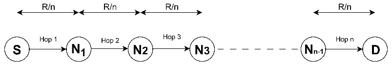 Figure 1. Multi-hop 1-D linear WSN model [7]
3. The Power Consumption Model Used
Wang et.al. [7] compared single-hop and multi-hop communication by using their own power consumption model and concluded that multi-hop communication is the optimal solution when sensor nodes are placed equidistantly between the source and destination nodes.
In this study, Mica2dot sensor nodes data and power consumption model proposed in [7] are used. The main difference of this model from the others in the literature is its dependence of the power amplifier performance which is drain efficiency (η).
There are some assumptions for this model. Communication bandwidth is so much low that interference and collisions could be avoided by using simple protocols without significant power consumption. Physical communication rate is assumed as constant.
The multi-hop power consumption over a given distance with equal hop distance between nodes is given in (1):
P(n) = (n-1)PR0+nPT0+[(nxεx(R/n)α)/η] (1)
n: number of hops
PR0: power consumption of a sensor node for receiving data
PT0: power consumption of a sensor node for transmitting data
ε: constant
R: distance between source and destination nodes
R/n: hop length
α: path loss exponent
η: drain efficiency (the ratio of RF output power to DC input
power)
Table 1 Typical values of path loss exponent [8]
| Environment | α |
| Free-Space | 2 |
| Urban area LOS | 2,7 to 3,5 |
| Urban area no LOS | 3 to 5 |
| Indoor LOS | 1,6 to 1,8 |
| Factories no LOS | 2 to 3 |
| Buildings no LOS | 4 to 6 |
The path loss exponent has different values depending on the
propagation environment as given in Table 1 [8]. In this study, the value for free space (α=2) is used.
4. Algorithmic Approach
The aim of the algorithm is to determine the optimum hop number at which minimum power consumption is obtained. The distance between the source and destination nodes is the input, the optimum hop number is the output of the algorithm. Optimum number of nodes, power consumption value at the optimum hop number, the required minimum number of hops and nodes are also given as the output at the end of the algorithm.
The flow diagram of the algorithm is given in Figure 2. The algorithm gets the distance between source and destination nodes as input. Minimum number of hop is obtained by dividing this distance to the Mica2dot sensor node maximum transmission distance. If the result is a non-integer number, it is rounded to the upper integer number and assigned to a variable. According to the power consumption model, the number of hop (n) is increased one by one starting from the minimum required hop number. The power consumption is calculated for each n. The number of hop and power consumption at this n are displayed on the screen every computation. The power consumption value for each n is compared to the one at the previous hop within the algorithm. If the previous power consumption is greater than current one, the computation is continued by increasing the n. When the computed power consumption value is firstly greater than the previous one, that critical point is determined as optimum hop number and the iteration is ended.
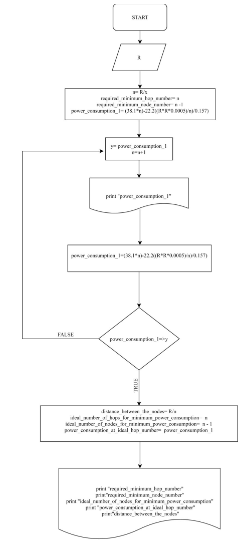 Figure 2. Flow diagram of the algorithm
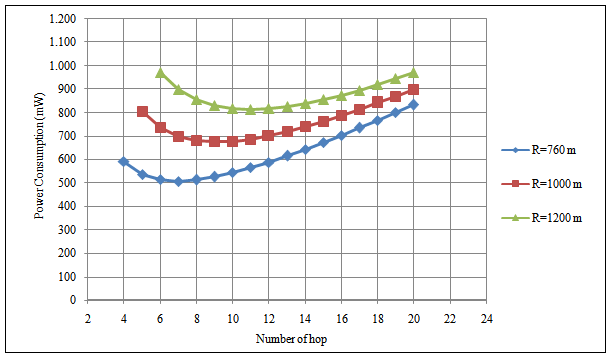 Figure 3. Power consumption versus number of hop
The distance between the source and destination nodes is asked by the algorithm. Then the beginning node number is computed by dividing this distance value to the node distance with maximum transmission power which is 230m for Mica2dot sensor node. The number of nodes is increased one by one from the starting value and iteration goes on until the minimum power consumption value is obtained. The power consumption decreases at first and it starts to increase after reaching its minimum value as expected from the results given in [8]. Since the minimum power consumption value is determined, no more calculation is required and the algorithm ends up.
During the development of this algorithm, Mica2dot sensor nodes are used [9] and Mica2dot sensor data is given in Table 2. However, this algorithm can be employed for any type of sensor node by using its hardware parameters or asking the required paramater values at the beginning as the input.
Table 2 Mica2 sensor node data
| PR0 | 22.2 mW |
| PT0 | 15.9 mW |
| η | 15.7 % |
| α | 2 |
| ε | 0.0005 |
For the distance between source and destination nodes as 760m, 1000m and 1200m, power consumption versus number of hop graph is obtained and given in Figure 3. When the number of hops is increased, the power consumption decreases at the beginning and then increases after reaching the minimum value.
This algorithm provides not only the optimum hop length and as a result optimum hop number but also the number of sensor nodes required for minimum power consumption directly without computing power consumption for each hop number.
5. Analytical Approach
As it is seen from Figure 3, the power consumption decreases at the beginning and then increases after reaching the its minimum value. Therefore, this is considered as mathematical issue finding minimum point and analytical approach is developed [1].
The hop number at which the minimum power is consumed is called as optimum hop number. Taking the derivative of (1) with respect to hop number, optimum hop number (nopt) is obtained as:
nopt = R{[η(PR0+PT0)]/[ε(-1+ α)]}-1/α (2)
For the α=2 value, (2) can be rearranged as:
nopt = R{[η(PR0+PT0)]/ε}-0.5 (3)
As it can be seen from (3), optimum hop number depends on sensor node receiving power (PR0), transmitting power (PT0), α, ε, η parameters and also the distance between source and destination nodes.
The optimum number of sensor nodes is defined as the sensor nodes required for minimum power consumption in a linear wireless sensor network with equidistantly placed sensor nodes. After optimum hop number is obtained, the optimum sensor nodes (dopt) can also be calculated by subtracting 1 from (3):
dopt= nopt -1 (4)
The more generic expression for optimum number of sensor nodes is given in (5).
dopt = R{[η(PR0+PT0)]/[ε(-1+ α)]}-1/α -1 (5)
Thanks to these mathematical expressions, the number of sensor nodes which are placed with equal hop length can be calculated directly from PR0, PT0, ε, η, α for a linear wireless sensor network.
6. Conclusion
WSNs can be deployed over the locations where are difficult to install traditional systems and this makes them attractive. On the other hand, sensor nodes are left unattended for a long period of time, lifetime of the network depends on how the limited energy supply of the nodes is used. Therefore energy efficiency issue is required to be considered during the application design. From the engineering design perspective, the aim of this study to determine the number of hops and sensor nodes for minimum power consumption in LWSNs including equidistantly deployed sensor nodes. For this purpose, both algorithm and analytical approaches are presented in this paper. Thanks to these approaches, the number of hops and thus the number of sensor nodes required for a LWSN application are determined according to the hardware parameters of the sensor nodes during design phase.
- N. Sazak and A. S. Kilinc, “Eşit Mesafeli Çok-Sekmeli Kablosuz Algılayıcı Ağlarda Minimum Güç Tüketimi için Optimum Düğüm Sayısının Belirlenmesi” in 2016 National Conference on Electrical, Electronics and Biomedical Engineering (ELECO 2016), Bursa, Turkey, 2016.
- I.F. Akyildiz, W. Su, Y. Sankarasubramaniam, “Wireless sensor networks: A Survey” Computer Networks, vol. 38, 393-422, 2002.
- M. Ilyas, I. Mahgoub, Handbook of Sensor Networks: Compact Wireless and Wired Sensing Systems, CRC Press, 2005.
- Y. Chen, Q. Zhao, “On the Lifetime of Wireless Sensor Networks,” IEEE Communication Letters, vol.9, no.11, 976-978, 2005.
- N. H. Mak, W. Seah, “How long is the Lifetime of a Wireless Sensor Network?” in International Conference on Advanced Information Networking and Applications, AINA’09, 2009.
- I. Jawhar, N. Mohamed, and D. P. Agrawal, “Linear wireless sensor networks: Classification and applications,” Journal of Network and Computer Applications, 34, 1671-1682, 2011.
- Q. Wang, M. Hempstead, W. Yang, “A Realistic Power Consumption Model for Wireless Sensor Network Devices” in Proc. 3rd Annual IEEE Communications Society on Sensor and Ad Hoc Communications and Networks, Reston, 2006.
- M. Kheireddine, R. Abdellatif, “Analysis of hops length in wireless sensor networks,” Wireless Sensor Network, 6(6), pp. 109–117, 2014.
- N. Sazak and A. S. Kilinc, “An Algorithm to Determine the Ideal Hop Length for Minimum Power Consumption in WSNs” in 2nd International Conference on Engineering and Natural Sciences (ICENS 2016), Sarajevo, Bosnia and Herzegovina, 2016.