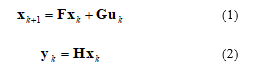
Image Navigation Using A Tracking-Based Approach
Image Navigation Using A Tracking-Based Approach
Volume 2, Issue 3, Page No 1478-1486, 2017
Author’s Name: Stephen Craig Stubberud1, Kathleen Ann Kramer2, a), Allen Roger Stubberud3
View Affiliations
1Advanced Programs, Oakridge Technology, San Diego, 92121, USA
2Department of Electrical Engineering, University of San Diego, San Diego, 92110, USA
3Department of Electrical and Computer Engineering, University of California, Irvine, 92697, USA
a)Author to whom correspondence should be addressed. E-mail: kramer@sandiego.edu
Adv. Sci. Technol. Eng. Syst. J. 2(3), 1478-1486 (2017); ![]() DOI: 10.25046/aj0203185
DOI: 10.25046/aj0203185
Keywords: Image correlation, Image navigation, Bearings-only tracking, Phase-only filter

Export Citations
Navigation is often performed using the Global Positioning Satellite system. However, the system is not always reliable for use at all times in all contexts. Reliance solely on such systems could endanger a vessel or get people lost. Another approach to provide navigation is to use known landmarks and triangulate one’s position. A navigation solution can be automatically generated using image data. In this paper, a target-tracking based approach for navigation using imagery is developed. The technique is based on an extended Kalman filter that uses angle measurements only. The technique is developed to use landmarks known a priori and landmarks that are first tracked by the vessel navigating and then used as known landmarks. The issues of observability to the development are considered. Image tracking from video frame to video frame is a further element. The frame-to-frame image correlation technique, the phase-only filter, is used to provide a low uncertainty estimate of the position of elements based upon the image frame. This provides an estimate of bearing angle that can be combined with a bearing from other known landmarks to fix and track the platform to provide a navigation solution.
Received: 31 May 2017, Accepted: 20 July 2017, Published Online: 10 August 2017
1. Introduction
Visual cues used in navigation have a very long tradition, as is evident from Homer’s The Odyssey [1],
At night he (Odysseus) never closed his eyes in sleep, but watched the Pleiades, late-setting Bootes, and the Great Bear that men call the Wain, that circles in place opposite Orion, and that never bathes in the sea. Calypso, the lovely goddess, had told him to keep that constellation to larboard as he crossed the waters.
Today, the primary navigational resource is GPS for systems from cell phones to vehicle navigation systems. In some cases, GPS signals are used to direct autopilot systems. But, at times, total reliance on GPS can be a detriment to navigation. There are places where the loss GPS can play havoc with a commuter. GPS signals are not available in urban canyons [2], such as in the heart of New York City or in Boston’s Ted Williams Tunnel near Logan airport.Besides the stars, landmarks such as Poseidon’s Temple at Cape Sunion, the Lighthouse of Alexandria, and the Roman lighthouse of Dover Castle provide testament to ancient use of upon a relative point. Using visual cues for navigation has long fixed reference points from which to understand location based been a standard procedure to ensure that ships could know where they were and get to desired locations.
GPS also can be jammed or spoofed. In [3], the weakness and danger of sole reliance on GPS was presented. In 2011, a United states spy drone was reported captured by Iran through jamming and spoofing of the GPS signal [4]. Even if untrue, the fact that it could be considered a plausible scenario, it shows the need for other navigation system in places when vessel or individual needs to navigate in precarious places.
For their submarine fleet, the uses “eyes-on” navigation and piloting for the ingress to or egress from a port. This kind of navigation of a submarine through the channel is both time and human-power intensive. This procedure uses a labor-intensive visual-based approach with a company of sailors stationed on the sail and hull of the vessel to point out channel markers, landmarks, and hazards. Information on what they see is relayed to the captain who can then act upon the information. Besides the potential dangers with relying on GPS, other navigation capabilities available to the submarine are not capable enough for navigation. Standard inertial navigation systems (INS are not currently accurate enough for such tight piloting [5]. Other types of sensors such as electromagnetic log and velocity sonar are unreliable in littoral conditions [5]-[7].
A number of techniques have been developed to overcome the issues that can arise relying solely on GPS navigation. Many incorporate inexpensive INS [2],[8]. It is well known, though, that these inertial systems have drifts and biases that without corrections will grow [8], [9]. For short periods of time and for operations where an human can control the motion of the navigating object easily, these systems are useful. To compensate for the drifts and biases, some of these non-GPS reliant navigators uses other sensors. In [10], the uses of imagery of the helmet that contains INS is used to compensate for the INS’s biases and drifts. Some systems, such as unmanned autonomous vehicles or drones, may be equipped with vision-based systems (video capabilities) rather than INS elements. In [11], [12] are typical techniques that use imagery for navigation. They use the image to provide a map over time. Complex image processing is then used to determine the relative position of the navigating object. In [13], [14], the concept of navigation using a target tracking approach based on the imagery was developed.
Unlike imaging techniques, such as [15], [16], the proposed method does not rely on an artifically-generated range estimate but instead on the angle-only information. Angle-only navigation is a common littoral navigation technique [17]. It is can also be considered the dual angle-only tracking [18]. In the tracking problem, the sensor platform has a known location and velocity while the targets’ kinematics are unknown. For angle-only navigation, landmarks with known fixed locatios are known. The sensor platform which wants to navigate uses its measured relationship to the landmarks to provide a crossfix of its positio. By repeating the crossfix estimate over time, a navigation track of the vessel can be computed. This method of navigation based upon tracking can handle obfuscation of individual landmarks, and can be used to locate new landmarks.
In [14], the concept of new landmarks being added to the existing set was discussed. That work is extended with the development of the approach and analysis of the performance.
In Section 2, the concept and effects of observability for angle-only navigation are presented. The use of the Phase-only Filter (POF) for the frame-to-frame image tracking and bearing generation is discussed in Section 3. Section 4 provides the improved navigation technique, including its functional flow. In Section 5, the bearings-only Kalman filter used within the technique is summarized along with the procedure to switch from tracking to navigation. Then this is then applied to frame-to-frame tracking in Section 6. An analysis of a simulation a maritime channel with multiple located landmarks some known and some unknown is provided.
2. Observability and Analysis Summary
2.1. Maintaining the Integrity of the Specifications (Heading 2)
The template is used to format your paper and style the text. All margins, column widths, line spaces, and text fonts are prescribed; please do not alter them. You may note peculiarities. For example, the head margin in this template measures proportionately more than is customary. This measurement and others are deliberate, using specifications that anticipate your paper as one part of the entire proceedings, and not as an independent document. Please do not revise any of the current designations.
Observability provides the ability to determine the state of system from the measurements. In [19], the standard observability Gramian for time-invariant linear system defined as
 was shown to be
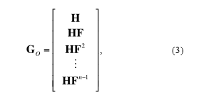 if Go is of maximal rank then the system is considered fully observable.
The image navigation problem defined for this problem is more complex. The measurement is defined as
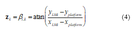 where the subscript LMi denotes the ith landmark that can be used by the sensor platform. As seen in Figure 1, the platform and two landmarks are present. The measurement to a single landmark is an angle, which is a nonlinear relationship from the landmark position and the platform position to the measurement space. As shown in [20], one way to obtain observability is to use multiple landmarks. This provides the well-known concept of a cross-fix as seen in Figure 1.
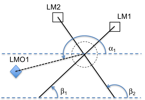 Figure 1. Example of creating a position of a nonsurveyed landmark to be used for crossfixing when one of the surveyed landmarks is no longer visible.
The navigation-solution initialization is created using bearing angles and knowledge of landmark locations:
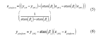 Since the horizontal location of the platform contains the information of both landmarks, only a single landmark’s information is necessary for the vertical component.
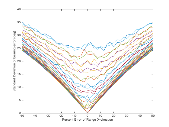 Figure 2 shows the old harbor entrance at La Rochelle, France. The two towers would be used as fixed landmarks on egress. The two channel markers in the front of the picture would make landmarks of opportunity as they are not as permanent structures as the towers would be.
For a landmark of opportunity, the structure being used must be fixed in position. The location of a fixed target can be determined by a moving platform. If the platform’s location is known at two time points, then the landmark of opportunity can have its position generated with a crossfix:
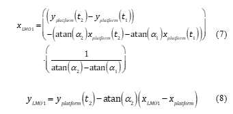 Crossfixing works very well for the case of small measurement uncertainties. However, since the platform is moving, a tracking algorithm, such as an extended Kalman filter (EKF) should be used to capture not only the position but the velocity dynamics. To capture the landmark of opportunity a tracking solution should also be used because of the uncertainty in the image sensor and the platform location. An EKF will smooth the error estimation noise than the single cross-fixes described in (5) – (8). To measure the observability of both the navigation solution and the landmark of opportunity position, the observability Gramian
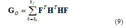 is used. Since the measurement is the bearing angle between the navigating platform and the ith landmark, bi from (13) and (14), the measurement-coupling matrix H becomes the linearized Jacobian of bearing angle with respect to each position’s coordinate direction of the platform position for navigation
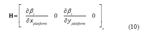 where the partial derivatives of each angle to the fixed, known ith landmark with respect to the platform coordinates is
 A similar Jacobian is generated with respect the landmark of opportunity’s position for the tracking problem.
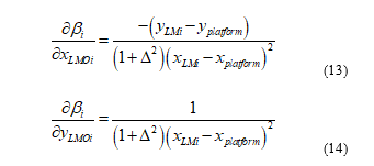 where D is defined as above.
The state-coupling matrix F is
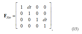 for the navigation solution, while it is defined as
 for the landmark tracking problem. The uncertainty of the sensor and platform location is incorporated by modifying (9) to be
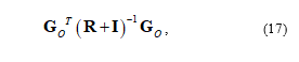
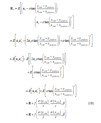 where R is the uncertainty covariance of the image measurement which models the sensor uncertainty. The added function f incorporates the uncertainty of the tion of the sensor platform (navigating vessel) for the Landmark of Opportunity tracking problem and, for the navigation problem, the Landmark of Opportunity’s own position uncertainty. This function is based on the estimated range from the navigating platform to the landmark and relative bearing from the navigating platform to the landmark. Since these two values are not known, they must be estimated from the filter solutions.
Figures 2 – 5 show the bearing uncertainty for four different relative platform-to-landmark angles. These angles are 0o, 30o, 60o, and 90o. The x-coordinate depicts the estimated position error of the platform (for tracking) or the landmark (for navigation) in relation to the actual range. The x-position error is in percent of the range. Figures 2-5 each depict 41 different plots corresponding to the range error in the y-direction. The range of error starts at -50% of the range and, in 2.5% steps, goes to 50% error in range.
These graphs were created by generation of 10000 Monte Carlo runs to compute the bearing error for each x-y position error. The plots indicate the expected symmetry in the position errors from -50% position error to +50% position error in each direction. As the position error in one direction gets smaller and nearer to direction of dominance (0o for the x-direction and 90o for the y-direction), the bearing error diminishes.
Figure 2. Bearing uncertainty (target is at 0o from the platform) based on the x-direction error in position.
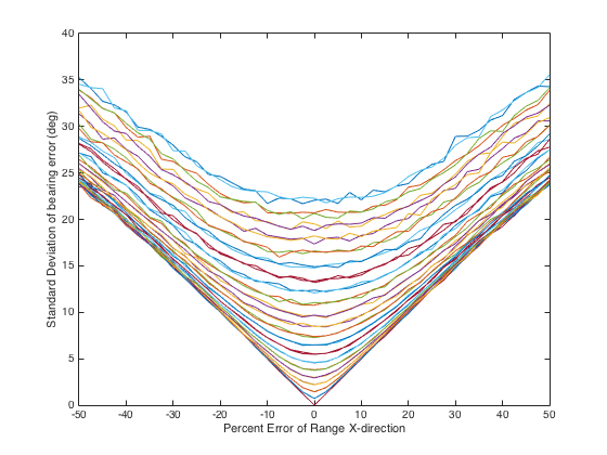 Figure 3. Bearing uncertainty (target is at 30o from the platform) based on the x-direction error in position.
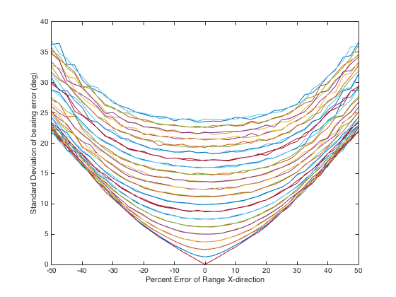 Figure 4. Bearing uncertainty (target is at 60o from the platform) based on the x-direction error in position.
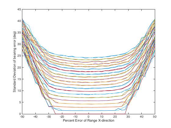 Figure 5. Bearing uncertainty (target is at 90o from the platform) based on the x-direction error in position.
3. The Phase-Only Filter
To generate the bearing measurements, the processor must know the orientation of the image sensor from the front of the navigating vessel. For a submarine this would be the rotation angle of the periscope from the bow of the submarine. This provides the center of the image frame. The landmarks in the image frame are then measured from the centroid to provide the angle adjustment from the pointing angle of the sensor.
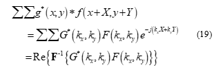
The approach that has been chosen to generate the image angle uses a two-dimensional image correlation process referred to as the phase-only filter (POF). The POF is a variant the Fourier correlation method. Using a two-dimensional Fast Fourier Theorem (FFT) algorithm, two images can be correlated element-by-element with speed and efficiency. Despite the large number of operations necessary to do such correlation, the process is still applicable to real-time situations. The frequency-domain version of the correlation function [21] is defined as (19):
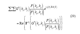
 While the FFT approach may seem useful, the actual physics of an image correlation problem using an optical correlator show that primarily the comparable information of images lies in the phase of the frequency information [21]. Mathematically this causes the amplitude information of the input image to be normalized. Thus, the correlation function becomes the phase-only filtered image correlation:
 The image correlation requires the template and the comparison image to be the same size, so padding the template image with zeroes to match the size of the scene image allows 2-D image correlation to indicate a match and also provides the location of the match within the scene.
For this application, the template would be the current image from the image sensor. While this seems backwards, the image being tracked is trying to be located in the image. As seen in Figure 6, Arabic letter pairs are being located on a license plate. The POF result of Figure 7 shows two peaks that align with the centroid of the letter pairs. The image angle will be computed as
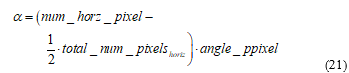 where the term angle_ppixel, the view angle per pixel, is computed from the optical view angle of the sensor and the number of pixels horizontally the sensor has:
 The input image is from a database or from the previous frame. The POF image correlation has been demonstrated to be a reliable technique to match and localize an object within a scene in many efforts [22]. In [14], the improved localization of the image correlation centroid, because of a sharper correlation peak, was shown than that for the straight FFT correlation method. This reduction in centroid area reduces the uncertainty of the total image uncertainty.
 Figure 6. Example of POF correlation. Two Arabic characters are looked for in a license plate. Two sets of the character pairs exist.
 Figure 7. POF correlation result in two correlation peaks located at the center of each character pair.
4. Image-Based Navigation
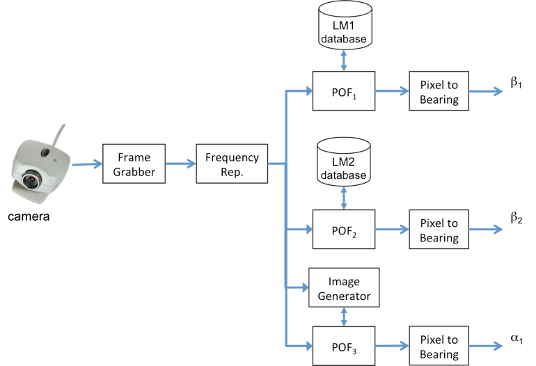 Figure 8 outlines the functional flow of the overall image-based navigation.
Figure 8. The functional flow of the image navigation system when unsurveyed landmarks are visible and can be used when surveyed landmarks are not available.
This section outlines the 10-step process, delving into the details of the components that this effort focuses on: image landmark tracking and image-based tracking. The steps are as follows:
Step 1: Initialize the navigation state of the platform. To determine which landmarks are surveyed in your database, a general knowledge of your location is required. This initialization need not be exact.
Step 2: Initialize the landmark database files. Once the known landmarks are defined, then the existing image databases for the local surveyed landmark positions are incorporated into the navigation algorithm.
Step 3: Grab the next video frame.
Step 4: Compute the angle of the electro-optical (EO) sensor with respect to the front of the vessel. This angle provides the relative angle of the center of the image with respect to the vessel.
Step 5: Correlate the known landmarks with the frame image. With the image data bases from Step 2 as the input to the POF algorithm and the video frame from Step 3 as the template, generate correlation peaks. If the peaks pass a predetermined threshold, the correlation peaks are considered a detection.
Step 5a: Calculate the angle of the landmark within the image. Using the computations from (21) and (22) for each correlation peak, the angle of the landmark with respect to the center of the image is computed.
Step 5b: Compute the landmark angle relative to the vessel. Add the angle from Stepb 5a to that of Step 4. This new angle is the measurement angle to the landmark.
Step 5c: Update or track image. As discussed in [13], the image is updated based on the previous frame to get a better aspect angle of the landmark for the next comparison. An image tracking algorithm can also be incorporated to estimate where the landmark should lie within the frame based on the estimated location of the vessel and the angle orientation of the sensor.
Step 6: Reinitialize the navigation solution with a crossfix. When two or more known landmarks are first available and their angles are computed, a crossfix initialization can be computed.
Step 7: Repeat Steps 5a – 5c. Start generating the angles for the navigation tracking algorithm.
Step 8a: Predict the estimation location of the vessel. Using the prediction equations of the EKF,
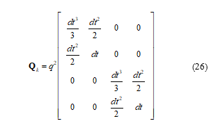
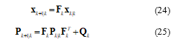 where x is the navigation state. The matrix P is the estimated error covariance of the state vector which indicates its quality. The state transition matrix F is defined in (15) while Q, the process noise is given as the integrated white noise process from [23],
 The location of where the vessel should be based on past measurements is the calculated result. This prediction takes the navigation estimate to the current time when a new measurement is available.
Step 8b: Update the estimation of the vessel’s location. Using the bearing measurements generated in Step 5b and the estimated location from Step 8a for computing the Jacobian, the location of the vessel is updated. The equations for the EKF are defined as
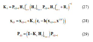 The matrix-vector K is referred to as the Kalman gain. The measurement uncertainty R is the composite measurement error defined in (18). The Landmark location is a fixed value. The superscript is used only in these equations to avoid confusion with the timing subscript.
Step 8c: If bearings of multiple landmarks are available, the update process of Step 8b is repeated. Since the landmarks are updated at the same time a zero-time-step prediction is used. This means that Step 8a is not repeated. Equations (28)-(29) are repeated but with the previously updated state values from the process of Step 8b.
Step 9: Define new landmarks of opportunity. As discussed with Figure 1, landmarks of opportunity are defined. Once identified, the image is placed in it own database.
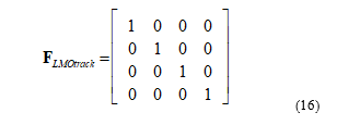
Step 10a: Track each landmark of opportunity. An bearing-only stationary tracking is implemented. The EKF for this application is defined as
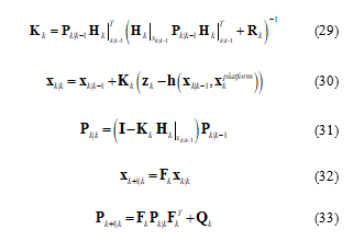 The Jacobian H is defined by (10) while the target kinematic dynamics FLMOtrack are defined by (16). The measurement uncertainty is defined not only by the sensor noise by also the location error of the navigation solution. The new measurement uncertainty R is calculated from (18).
Step 10b: Incorporate the new landmark into the available set. After the landmark has reach an acceptable level of accuracy, the tracking algorithm is stopped. The measurement noise is updated using (18). This measurement noise is used throughout the use of the new landmark. The new landmark and associated measurement noise is then used in Step 3 – 9. Note that a landmark of opportunity cannot be used in the initialization step as that would contain too many unknowns to solve the location calculations.
5. Analysis Scenario
In [14], a scenario using road data along United States Interstate 15 in the state of California was demonstrated to provide excellent performance when surveyed landmarks were available. In this effort, the analysis extends to a simulation of what occurs when landmarks of opportunity are incorporated into the scenario.
The example is a variant of the scenario developed in [20]. The scenario simulates a simple port entry and is illustrated in Figure 9. A platform wishing to use angle-only navigation heads north for 1000 s at 4.0 kts. The platform then heads east for 500 s at 4.0 kts. The platform starts at location 0, 0. There are four landmarks, Landmarks 1 – 4 in order are located at positions (1.5 nmi, 0.6 nmi), (0.375 nmi, -1.25 nmi), (0.5 nmi, 1.5nmi), and (2.2 nmi, -1.125 nmi), respectively. Landmarks 1 and 2 are defined as known landmarks with pre-surveyed locations. Landmarks 3 and 4 are defined as landmarks of opportunity. A 5.0o Gaussian random error was placed on each bearing measurement as the sensor component of the error.
After 60 seconds, the vessel starts tracking Landmarks 3 and 4 as landmarks of opportunity. This tracking continues to 850 seconds. After that point, the landmarks of opportunity are used with Landmarks 1 and 2. After 1000 seconds into the scenario, Landmarks 1 and 2 are no longer used. Only Landmarks of 3 and 4 are used through the rest of the scenario.
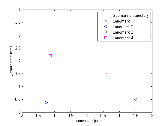 Figure 9. A Simple Scenario of a Submarine Navigating with Potentially Four Landmarks.
6. Analysis Results
The tracking error estimate provides approximately a 3.0% of error in the x-direction and 3.5% error in the y-direction for Landmark 3. For Landmark 4, a 2.0% error and 2.2% error in the x and y directions, respectively are generated. Using the results in Figures 2 and 3, the added bearing error is approximately a 2.1o error. This makes the matrix R increase from 0.0076 radians-squared to 0.0090 radians-squared using (18). The tracking solution for Landmark 3 is tracked to be at position (0.492, 1.488). The tracking solution for Landmark 4 is tracked to be at position (2.296, -1.232).
The uncertainty for Landmark 3 navigation is defined as 23% for each direction. This results in a 12o added error to the measurement uncertainty. For Landmark 4 uncertainty in position is 4% and 4.5% in relation to the range in the x and y directions, relatively.
The results of the navigation accuracy are shown in Figure 10. As clearly seen, the navigation error is quite small when the surveyed landmarks are used. When only the landmarks of opportunity are used, error spikes appear. Deeper analysis indicates there are two reasons for this. The first is that Landmark 3 has too great of an uncertainty in its tracked location for it too be very effective. The second is that, at times near the end of the scenario, Landmarks 3 and 4 align reducing the observability.
The analysis indicates that the landmarks of opportunity require that the a figure of merit be used to determine if such a landmark is viable for navigation purposes. Also, the angular disparity between two landmarks is a necessary decision in selection.
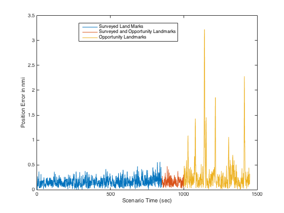 Figure 10. Position error of the navigation solution for three segments of the scenario: two surveyed landmarks, two surveyed landmarks and two landmarks of opportunity, and two landmarks of opportunity.
7. Conclusions
An image-based navigation system was developed using a bearings-only tracking system. The technique uses image correlation to measure the bearings by fixing on visible surveyed landmarks. The initial simulations and the test case have shown that this technique has merit as a navigation approach for ingress and egress operations where more standard forms of navigation are not available but surveyed locations in the region are. Tracking potential landmarks of opportunity can help if the tracking solutions are a quality level of accuracy.
In the next phase of this system’s development, maritime data will be collected and utilized in testing. The results of this paper also indicate the need to develop figure of merit tool to determine if landmarks of opportunity can be incorporated into the approach.
Conflict of Interest
The authors declare no conflict of interest.
- A. T. M. Homer, George E. Dimock, The Odyssey. Cambridge, MA: Harvard University Press, 1995.
- W. Soehren and W. Hawkinson, “Prototype personal navigation system,” IEEE Aerospace and Electronic Systems Magazine, vol. 23, no. 4, pp. 10-18, April 2008. https://doi.org/10.1109/MAES.2008.4493437
- T. E. Humphreys, “Statement on the vulnerability of civil unmanned aerial vehicles and other systems to civil GPS spoofing,” Subcommittee on Oversight, Investigations, and Management of the House Committee on Homeland Security, 2012.
- J. Leydon, “Iran spy drone GPS hijack boasts,” The Register, 2013.
- H. Rice, S. Kelmenson, and L. Mendelsohn, “Geophysical navigation technologies and applications,” in Proceedings of the Position Location and Navigation Symposium – 2004. IEEE, pp. 618-624. https://doi.org/10.1109/PLANS.2004.1309051
- I. B. Vaisgant, Y. A. Litvinenko, and V. A. Tupysev, “Verification of EM log data in marine inertial navigation system correction,” Gyroscopy and Navigation, vol. 2, 2011, p. 34-38. https://doi.org/10.1134/ S207510871101010X
- R. A. Smith, L. Russell, B. D. McKenzie, and D. T. Bird, “Synoptic data collection and products at the Naval Oceanographic Office,” in OCEANS, 2001. MTS/IEEE Conference and Exhibition, vol. 2, 2001, pp. 1198-1203. https://doi.org/10.1109/OCEANS.2001.968283
- S. Moafipoor, D. A. Grejner-Brzezinska and C. K. Toth, “Multi-sensor personal navigator supported by adaptive knowledge based system: Performance assessment,” 2008 IEEE/ION Position, Location and Navigation Symposium, Monterey, CA, 2008, pp. 129-140. https://doi.org/10.1109/PLANS.2008.4570049
- A. Kealy, N. Alam, C. Toth, T. Moore, et al, “Collaborative navigation with ground vehicles and personal navigators,” in 2012 International Conference on Indoor Positioning and Indoor Navigation (IPIN), Sydney, NSW, 2012, pp. 1-8. https://doi.org/10.1109/IPIN.2012.6418893
- M. Harada, J. Miura and J. Satake, “A view-based wearable personal navigator with inertial speed estimation,” in 2013 IEEE Workshop on Advanced Robotics and its Social Impacts, Tokyo, 2013, pp. 119-124. https://doi.org/10.1109/ARSO.2013.6705516
- D. Bradley, A. Brunton, M. Fiala and G. Roth, “Image-based navigation in real environments using panoramas,” in IEEE International Workshop on Haptic Audio Visual Environments and their Applications, 2005, pp. 57-59. https://doi.org/10.1109/HAVE.2005.1545652
- P. Lukashevich, A. Belotserkovsky and A. Nedzved, “The new approach for reliable UAV navigation based on onboard camera image processing,” in 2015 International Conference on Information and Digital Technologies, Zilina, 2015, pp. 230-234. https://doi.org/10.1109/DT.2015.7222975
- T. C. Glaser, N. Nino, K. A. Kramer and S. C. Stubberud, “Submarine port egress and ingress navigation using video processing,” in 2015 IEEE 9th International Symposium on Intelligent Signal Processing (WISP) Proceedings, Siena, 2015, pp. 1-6. https://doi.org/10.1109/ WISP.2015.7139153
- S. C. Stubberud, K. A. Kramer and A. R. Stubberud, “Navigation using image tracking,” in 2016 IEEE International Conference on the Science of Electrical Engineering (ICSEE), Eilat, Israel, 2016, pp. 1-5. https://doi.org/ 10.1109/ICSEE.2016.7806050
- Z. P. Barbaric, B. P. Bondzulic, and S. T. Mitrovic, “Passive ranging using image intensity and contrast measurements,” Electronics Letters, vol. 48, pp. 1122-1123, 2012. https://doi.org/10.1049/el.2012.0632
- M. Hirose, H. Furuhashi, and K. Araki, “Automatic registration of multi-view range images measured under free condition,” in Proc. of the Seventh International Conference on in Virtual Systems and Multimedia, 2001, pp. 738-746. https://doi.org/10.1109/VSMM.2001.969738
- F. J. Larkin, Basic Coastal Navigation: An Introduction to Piloting. Dobbs Ferry, NY: Sheridan House, 1998.
- S. S. Blackman, Multiple-Target Tracking with Radar Applications. Dedham, MA: Artech House, 1986.
- M.S. Santina, A.R. Stubberud, G.H. Hostetter, Digital control system design, Saunders College Pub., 1994.
- S. C. Stubberud and K. A. Kramer, “Navigation using angle measurements,” Mathematics in Engineering Science and Aerospace (MESA), 8(2), 201-213, 2017.
- C. J. Stanek, B. Javidi, A. Skorokhod, and P. Yanni, “Filter construction for topological track association and sensor registration,” in Proc. of SPIE, 2002, pp. 186-202. https://doi.org/10.1117/12.467794
- E. Ramos-Michel and V. Kober, “Correlation filters for detection and localization of objects in degraded images,” in Progress in Pattern Recognition, Image Analysis and Applications. vol. 4225, J. Martínez-Trinidad, J. Carrasco Ochoa, and J. Kittler, Eds., ed: Springer Berlin Heidelberg, 2006, pp. 455-463. https://doi.org/10.1007/11892755_47
- Y. Bar-Shalom, X.-R.K.T. Li, Estimation with applications to tracking and navigation, Wiley, 2001.