1.    Introduction

      This paper is an extension of work originally presented in The 15th IEEE International Conference on Machine Learning and Applications [1]. Genome mapping [2] is the process of finding the order of markers within chromosomes; where markers are short fragments of Deoxyribo Nucleic Acid (DNA) sequence most often located in noncoding regions of the genome (regions that do not encode protein sequences). Markers orders can provide researchers with essential information for localizing disease-causing genes in the genome. Radiation Hybrid (RH) Mapping [3] is a statistical mapping technique to order markers along a chromosome, and estimate the physical distances between markers. RH mapping is  widely used in many mapping projects, and has several advantages over alternative mapping techniques [4]. In RH Mapping, chromosomes are separated from one another, then high doses of X-rays are used to break the chromosome into several fragments. The main principle of RH mapping is that the probability of separation of two adjacent markers due to radiation breakage increases with the increase in physical distance [4]. The order of markers on a chromosome can be calculated by estimating the frequency of breakage and retention between the markers.

An RH population can be seen as a m X n Boolean matrix, where m is the number of markers, and n is the number of individual organisms in the mapping population. A single RH vector represents one marker across all individuals/Panels. All markers in each panel is assigned a value of 1 or 0, where the value 1 indicates the presence of that marker in that panel, and the value 0 indicates the absence of that marker. Once all markers in all panels are screened and saved, the RH population will be used for the mapping process. Figure 1 shows a sample RH population of 3 markers on 6 panels.

The toy example in Figure 1 is used just to explain the process of mapping a RH population. Typically, the number of markers in chromosomes range between a hundred to thousands. Thus, calculating the OCB for all markers permutations is unfeasible solution for such large numbers of markers; where for n markers, there are n!/2 permutations to evaluate. In this study, we are going to map a RH dataset of the human genome with hundreds of markers. Heuristic approaches [6-8] have been used to map such larger datasets of markers in a reasonable time. Although the heuristic approaches are relatively fast, they scale exponentially with the number of markers. Figure 2 shows the typical pattern of mapping different datasets of markers using some heuristic algorithms that have been used to map RH populations in many researches [9-12].After preparing the RH population, the RH mapping process starts. The Obligate Chromosome Breaks (OCB) is used to indicate the similarity and estimate the distance between two markers in RH population [5]. The basic mapping step is to estimate the OCB between all pairs of markers, where a 1 is followed by 0 or vice versa in the same panel, and place the closest (similar) markers together. For example to map the simple population in Figure 1, we need to find the similarity between these three RH vectors (markers), and then place the similar markers close together in the constructed map. First calculate the OCB for all possible markers permutations (the number of times a 1 is followed by 0 or vice versa in the same panel), and second select the permutation with the minimum number of OCB; the best map of these three markers is {M1, M2, M3} with five breaks. Any other permutation will have more than five breaks.

The main goal of this study is to propose an alternative approach to map large numbers of markers in a short time. The proposed approach works in two phases. Phase 1, has been originally published in [1], constructs maps as follows: 1) Uses Jackknife resampling method on the original RH population to  create slightly variant RH samples. Then, all the generated samples are grouped into clusters based on their LOD (logarithms of odds -base 10) scores. The LOD score [14] was developed as a probabilistic measure for linkage, and has been used consistently throughout the RH literature [9-11]. 2) Merges all RH samples clusters into consensus clusters, and filters out the unreliable markers. 3) Constructs a map for each consensus cluster. 4) Connects all consensus clusters maps into one single map. Phase 2, uses the output map of Phase 1 as a skeleton to map additional markers and improve the resolution of the initial map. Phase 2 works as follows: 1) Uses Kmeans clustering to find the candidate markers to be added to the map. 2) Finds the best position of each candidate marker in the initial map in order to add them to improve the final constructed map.

To demonstrate the effectiveness of our approach, three metrics are going to be used: 1) Accuracy, which indicates the agreement of the constructed maps with the published maps. 2) The number of mapped markers in the constructed maps. 3) The running time to construct the maps. We will compare our constructed maps with the maps we published in our original work in [1]. Also, we will compare our results with a state-of-the-art tool for building radiation hybrid maps. In our approach, we use the Clustering technique to reduce the mapping computational complexity, thus, mapping large datasets of markers in a short time. Also, our approach considers the problem of noisy markers and can filter out unreliable markers to increase the accuracy of the constructed maps.

The rest of this paper is structured as follows: Section 2 presents the related work. In Section 3, our proposed approach is discussed in detail. Section 4 presents the experimental results of the proposed approach, and Section 5 concludes this research.

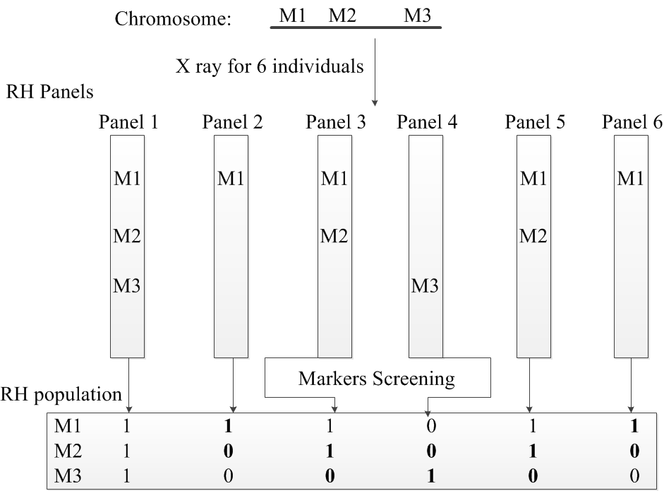Figure 1. A toy example of an RH population for 3 markers on 6 panels. Breakages are highlighted in bold.

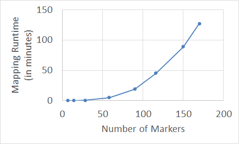Figure 2. Relationship between No. of markers and mapping complexity using heuristic algorithms implemented in the Carthagene tool.

2.    Related Work

Conventional techniques [15, 16] for filtering out unreliable markers depend mainly on resampling [17]. Thus, these  techniques are not recommended for filtering out unreliable  markers from a large dataset due to their high computational complexity. The filtering process can be summarized in three sequential steps: 1) Resample the original dataset. 2) Use mapping techniques to map each resampled dataset. 3) Construct a matrix to show the reliability of all markers and filter out the most unreliable marker. These three steps are repeated to filter out unreliable markers one at a time. This iterative process is too time consuming for a large dataset, as to filter out only one unreliable marker, there is a need to resample the dataset and map all resampled datasets. The computational complexity of mapping a single resampled dataset scales exponentially with the number of markers to be mapped, as shown in Figure 2. Thus, repeating this complex mapping process for every single resampled dataset to filter out one unreliable marker is not a feasible solution for large datasets. As we discuss our proposed solution in Section 3, we will show that how our approach resampled the dataset and filtered out the unreliable markers without the need of mapping the resampled datasets. Thus, the proposed approach reduces the computational complexity of the whole mapping/filtering process.

RHMapper tool [12] provides another approach to build solid maps with only the reliable subset of markers. The mapping  process  is  divided  into  two  steps:  1)  use find_triples command to search the data set for well-ordered triples, and save them. 2) Use assemble_framework1 or assemble_framework2 commands to assemble the saved well-ordered triples into a final map. The assembly process uses the overlapping between the well-ordered triplets of markers to combine them into a final map, where the assemble_framework1 command seeks for overlapping with two consecutive markers in each triplet, for example: triplets (A-B-C) and (B-C-D) will be assembled into (A-B-C-D). assemble_framework2 command can add gaps to assemble triplets, for example: triplets (A-B-C) and (A-C-D) will be assembled into (A-B-C-D). Although, this mapping strategy can build solid maps, mapping a hundred markers takes several hours to finish [13], so this approach does not scale well with the number of markers.

Multimap [13] is another tool to build maps with reliable markers. The mapping process starts with searching for the strongest pair of markers, then iteratively adds one marker at a time to extend the initial map. Apparently, this mapping process does not scale well with large datasets of markers.

Carthagene tool [11] is another well-known package that has been used in many studies to construct solid maps [24, 25]. The Buildfw command implements an incremental insertion procedure to build maps with only reliable markers; and it works as follows: first, search for the triplet of markers that maximizes the difference between the likelihood of the best map, and the second best map using only this triplet of markers. Once the best triplet of markers is found, save it as an initial framework map. Second, for each marker not mapped in the framework, try to insert it into its best interval. In order to insert a marker into its best interval in the framework map, two thresholds are evaluated: 1) AddThres and 2) KeepThres. AddThres is used to determine if a marker can be placed in its best interval or not; where if the loglikelihood difference between the best two insertion intervals is greater than the AddThres, then the marker can be inserted in its first best interval in the map. If that marker can be inserted in its best interval in the map, the KeepThres is evaluated, which is used to determine if the new inserted marker can be saved in the framework map or not. If the loglikelihood difference between the best two maps is greater than the KeepThres, then the new inserted marker will be saved in its best interval and will be used to map other markers in the following iterations. Otherwise, the new inserted marker will be removed from the current framework map.

One of the limitations of the incremental insertion procedure in Carthagene is that only a few markers are mapped at the final map, if the recommended values of the AddThres and KeepThres are used [11]. Another limitation is that the mapping process starts with only three markers as an initial map. Thus, adding one marker at a time to the initial map makes the mapping process not suitable for large numbers of markers. Moreover, the incremental insertion procedure cannot be parallelized.

In this research, we compare our proposed approach with the Carthagene incremental insertion approach. Our proposed approach can take advantage of the parallel computing to reduce the computation complexity of the mapping process; where markers are grouped into smaller clusters, and these groups of markers can be mapped in parallel. We expect to outperform the Carthagene approach in terms of the mapping runtime. Also, in terms of mapping accuracy, our proposed approach uses the grouping process over all resampled data to filter out the unreliable markers, and thus uses only the reliable markers to build solid final maps. We expect our approach to build solid maps, as the grouping process will help in reducing the effect of unreliable markers to the local clusters maps, not to the entire map.

3.    Proposed Approach

The proposed approach divides the mapping process into two phases, where each phase consists of several steps. The first phase builds an initial map with the most reliable set of markers, Figure 3 shows the systematic workflow of the first phase. The second phase uses the initial map constructed in phase 1 as a framework to map more markers to the initial framework, which results in building a high resolution map (mapping larger numbers of markers), Figure 4 shows the systematic workflow of the second phase

3.1.  Phase 1: Building Initial Framework Map

• Resamplingand grouping: The Jackknife resampling technique is used to generate N variant RH samples of the original RH dataset, where each resampled RH dataset will haveN-1 individuals (leave-one-individual-out).f After generating the resampled datasets, the Single Linkage Agglomerative Hierarchical clustering technique [18] is used to group each dataset into different clusters of markers. The group command is implemented in the Carthagene tool can be used to create these clusters of markers. The idea of the grouping is to create small groups of markers with low intra-cluster distances and high inter-cluster distances.

 Groups aggregation and filtering: The first step generates N variant RH sampled datasets, and with each resampled dataset many clusters of markers. The goal of this step is to use all clusters of markers of all resampled datasets to filter out unreliable markers and aggregate the clusters of markers to generate solid consensus clusters. A matrix of size m x m is used to show the stability of linkage relationship between all pairs of markers, where m is the number of markers in the RH population. The matrix is created and initialized to Zero. Then, we trace all the clusters in all RH sampled datasets to update the values of the elements of the matrix. For each paired ordered markers (Mi, Mj), we increment both indexes (i, j) and (j, i) in the cluster matrix by 1 each time the pair (Mi, Mj) appear in one cluster in all sampled datasets.

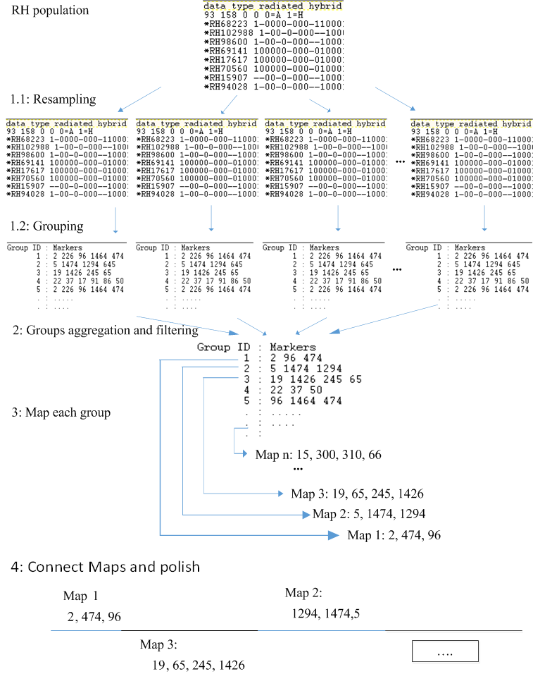Figure 3. The proposed algorithm for building initial framework maps.

After that, we start filtering out unreliable markers; two factors are defined for each marker: 1) the Stability-Factor (SF), which indicates the stability of neighbors markers throughout all sampled datasets clusters. For example, the Stability-Factor value of 80 for markers (Mi, Mj) means that over all resampled RH datasets, markers (Mi, Mj) appear 80 times together in the same cluster. 2) The Reliability-Ratio (RR), which is calculated by the count of relationships above the Stability-Factor divided by the total number of relationships for that marker. Figure 5 shows a simple example to illustrate the filtering process. All markers with Reliability-Ratio less than a threshold are considered unreliable markers and can be filtered out. In our experiments, we used RH population of 93 individuals and filtered out markers with SF values less than 80, and RR less than 50%. After filtering out the unreliable markers from all clusters, the remaining markers will be considered reliable markers and will form the consensus clusters.

• Mapping clusters’ markers: In this step, we build a map for each consensus cluster of markers. Several heuristics algorithms can be used to build the maps, in this study, we follow the mapping strategy published in [4, 9,10] to build a map for each cluster, using the heuristics algorithms implemented in the Carthagene tool [11]. The following steps present the mapping strategy: 1) Mrkdouble command to identify and merge identical markers by a single marker. 2) Build command to build an initial nice map, where the command finds the best pair of markers, with the strongest linkage, and incrementally tries to add the remaining markers if they satisfy the insertion criteria. 3) Greedy and Annealing commands are used as improvement steps to find a better map in case a local improvement exists. 4) Flips and Polish commands are used to apply all possible permutations in a sliding window to check if a better map can be achieved. Running all these commands in that sequence will build a map for each cluster.
• Connect maps and polish: Building a map for each consensus cluster shows the local order of the markers in each cluster. However, all these small maps need to be concatenated to form a whole chromosome map. In this step, we concatenate the clusters’ maps generated in the previous step to form one map for a whole chromosome. This process can be done in an iterative manner.First, we extract the boundaries, the first and the last marker, of each cluster map. Second, we group all boundaries into clusters, the group command in Carthagene can be used to make these clusters; we start with a high LOD score T, i.e. T= 18. Boundaries from different maps that fall into one cluster are connected using the closest boundaries to form a bigger map. This step is repeated, where at each iteration the LOD score T needs to be lowered by a factor of x, i.e. x= 3, to let the far away boundaries to be connected to form one single map. A polishing step is used at the end of this step to improve the constructed map by trimming marker at the edges of the final map with LOD score less than 3, which generally indicates that there is no linkage between two markers.

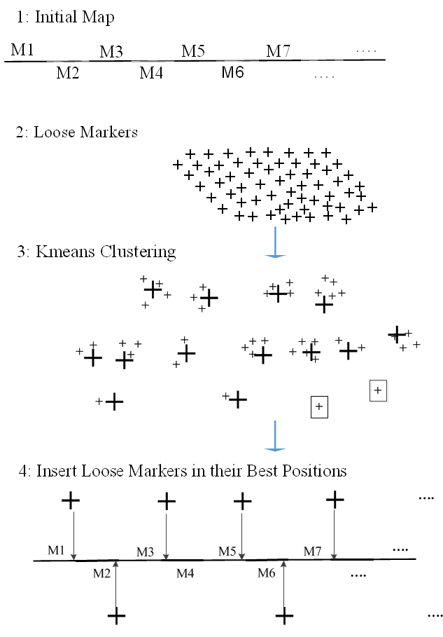Figure 4. The proposed algorithm for improving the initial framework maps.

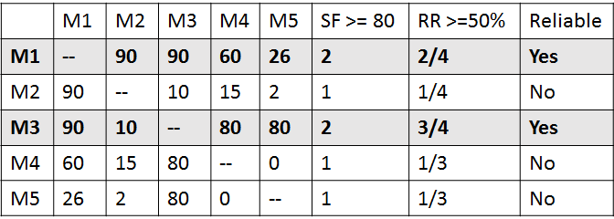Figure 5. A simple example to illustrate the filtering process: Markers M1 and M3 are defined as reliable markers.

3.2.  Phase 2: Improving Framework Map

• Loose markers extraction and grouping: After building a framework map with only the most reliable subset of markers, our goal is to use the framework map as an initial map to construct a high resolution map by mapping more markers from the remaining left out markers (Loose Markers) to the initial framework map. In this step, we use the initial constructed framework map as a skeleton to map the loose markers, where loose markers will be placed into the intervals of the initial framework map. This process works as follows: 1) Extract the loose markers from the original dataset. 2) Group the loose markers into clusters; the Kmeans algorithm is used to make the clusters of the loose markers. Kmeans algorithm works well for large datasets. To run the Kmeans algorithm, we need to set the number of clusters (K). In this study, we set the value of K to the number of markers in the initial framework map plus 1. Assuming that all loose markers are going to be placed in between framework’s markers, so if the number of markers in the framework map is n, that means we have n+1 number of intervals to place the loose markers in. Thus, the number of clusters K can be set as n+1, if the number of loose markers is less than the number of markers in the initial framework map, then we consider each loose marker as a single cluster.
• Insert loose markers in their best positions: The kmeans algorithm will group the loose markers into clusters, where markers within clusters are too close to each other and far away from other clusters’ markers. Generally, for large datasets singleton clusters, clusters with only one marker, are considered unreliable clusters and will be filtered out, as they are not attached to any other loose markers. After we group the loose markers into clusters, we choose randomly a loose marker from each clusterand try to place that loose marker into its best position in the initial framework map. To find the best position of that loose marker, the Buildfw command in Carthagene is used to report the best position for each loose marker, where the loose marker is inserted in all possible positions in the framework map, and then reports the best position based on the linkage of the loose marker with its immediate neighbors (left and right markers, if possible). After we find the best position of each loose marker, we add them to their best positions. In case there are more than one loose marker in one position, we randomly pick one marker and keep it in that position. Step 1 and Step 2, in Phase 2, can be repeated to include more markers in the framework map, where the final map of each iteration is used as an input for the next iteration to map as many loose markers as needed. Figure 4 shows the systematic workflow of Phase 2.

4.    Experimental Results

4.1.  Datasets

The three common used human genome radiation hybrid panels are: 1) The G3 [19] and 2) TNG [20] panels produced by Stanford University and 3) The Genebridge 4 [21] panel by the Sanger Center. In this study, we use the Genebridge 4  panel where the number of individuals is 93. We have selected 8 different chromosomes with varying number of markers to show the scalability of our proposed approach over the increasing number of markers. Table 1 shows the selected chromosomes with their numbers of markers. The choice of these chromosomes is determined by the availability of markers in both radiation hybrid data set and physical marker locations. The physical marker locations are extracted from the Ensemble website [22], and the RH dataset are downloaded from the EMBL-EBI website [23].

4.2.  Evaluation of the approach

The proposed mapping approach builds maps in two phases: In Phase 1, we construct initial map with the most reliable markers. Once the initial map is constructed, Phase 2 extends the initial map to include more markers in the final map. In this section, we are going to refer to Phase 1 as Clustering Method; and Phase 1 and Phase 2 together as Extended Clustering Method. The Clustering Method has been evaluated in [1], where the reported results show that the constructed maps have high agreement with the corresponding physical maps. To evaluate the Extended Clustering Method, we use the same dataset we have used in [1], the constructed maps reported in [1] will be used as an input to Phase 2 in the Extended Clustering Method.

The running time for the Clustering Method has been reported in [1] and can be seen in Figure 6. The big improvement in the mapping runtime of our Clustering Method over the Carthagene Method can be explained by the grouping of the large numbers of markers into small groups, and taking advantage of parallel processing to map all these groups of markers simultaneously in a short time. The hieratical clustering in the Clustering Method and the Kmeans clustering in the Extended Clustering Method only take a few seconds to complete. On the other hand, the Carthagene Method, uses only three markers as an initial map and then incrementally adds more markers to that initial map one marker at a time to construct the maps. Figure 6 shows the mapping running time for both Carthagene Method and the Clustering Method using the same dataset. The Extended Clustering Method running time depends on two factors; first, the numbers of markers in the initial map, and second, the number of iterations; where the more markers there are in an initial map, the less time it takes to map the remaining markers. Table 1 shows that the Clustering Method can generate initial maps with large numbers of markers compared to the number of markers in the maps constructed using the Carthagene Method.

The accuracy of the constructed maps is measured by Pearson Correlation, where the closer the value is to 1, the stronger the linear correlation (agreement) between the markers positions in the constructed maps, and the markers positions in the corresponding physical maps. Table 1 shows the Pearson Correlation between the  physical  maps and the constructed maps using 1) Carthagene  tool;  2) The Clustering Method; and 3) The Extended Clustering Method. The results show that maps generated using the Clustering Method have higher correlations with the physical maps than the maps generated using the Carthagene tool. Out of 10 chromosomes, the Carthagene tool outperforms the Clustering Method for only one chromosome, Chromosome 21, with a slight difference. While, the Clustering Method outperforms the

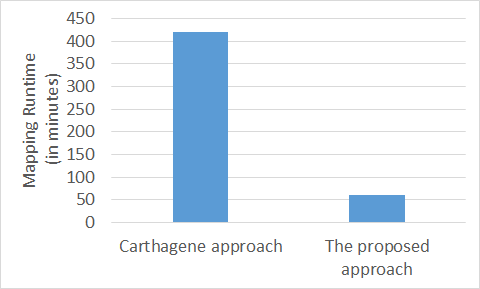Figure 6. The proposed approach mapping runtime vs the traditional Carthagene approach.

remaining 9 chromosomes. For some chromosomes the improvement is huge, for example, Chromosome 3, the accuracy of the Carthagene Method is 0.45 while the accuracy of the Clustering Method is 0.99. Another example is Chromosome 12, where the accuracy of Carthagene Method is 0.10, while the accuracy of Clustering method is 0.73. For some other chromosomes, the difference in accuracy between the Carthagene Method and Clustering Method is small, for example: Chromosome 10, the accuracy of Carthagene Method is 0.98, while the accuracy of the Clustering method is 0.99. Also in Chromosome 21, the accuracy of Carthagene Method is 0.98, while the accuracy of Clustering method is 0.97.

Moreover, Table 1 shows the number of mapped markers in each chromosome using all three methods. The results show that for most chromosomes the constructed maps using the Clustering Method have more markers than the constructed maps using the Carthagene Method. One of the limitation of the Carthagene Method is that the constructed maps have only a few numbers of markers, and this can be seen in Chromosomes 10 and 12. For Chromosome 10, Carthagene maps only 16 markers, where the Clustering Method maps 46 markers. For Chromosome 12, Carthagene maps 42 markers, while the Clustering Method maps 71 markers. For other chromosomes the numbers of mapped markers between the Carthagene Method and The Clustering Methods are similar and this can be seen in Chromosome 16, 21 and 22 where the difference in mapped markers is small. In some cases, Carthagene tool maps more markers than the Clustering Method, for example Chromosome 3 and 7. However, the correlations between the constructed maps and the physical maps for these chromosomes are not as strong as our proposed approach maps for the same corresponding chromosomes.

Table 1- Comparison Of The Number Of Mapped Markers And Correlation Between The Constructed Maps And The Physical Maps For Carthagene Method, Clustering Method, Extended Clustering Method.

      The main goal of the Extended Clustering Method is to map more markers to build high resolution maps. The Extended Clustering Method is an iterative process, where in each iteration some markers are added to the current map to form a new map, and that new map will be used in the next iteration to map more markers, and so on. Table 1 shows the number of mapped markers for each chromosome using the Extended Clustering Method for one iteration. For Chromosome 3, the Extended Clustering Method mapped 215 markers, while the Clustering Method mapped 153 markers. Although, the number of mapped markers is increased in the Extended Clustering Method map, the accuracy of the constructed map remains high 0.99. The same pattern is shown for Chromosome 18. For other chromosomes, Chromosomes 5 and 7, the number of mapped markers is increased and the accuracy of the final maps is decreased slightly. In other cases, for example Chromosome 12, The Extended Clustering Method mapped more markers, but the accuracy dropped from 0.73 to 0.68. Although the accuracy of Chromosome 12 was dropped to 0.68, it is still higher than the accuracy of the Carthagene map, 0.10.

To  show  graphical  representations  of  the  alignment  of the constructed maps for some chromosomes using both the Carthagene Method and the Extended Clustering Method, we plot the known markers positions along the x-axis, and the predicted markers position along the y-axis. The plots show how well the constructed maps agree with the corresponding physical maps. The diagonal line in each plot shows the perfect alignment between the predicted markers positions and the actual markers positions. Figures 7 to 22 show the maps for all 10 chromosomes. Our approach is designed to build robust maps. The resampling and clustering techniques are intended to filter our unreliable markers and map only reliable markers. Moreover, mapping markers inside a cluster does not affect the mapping of the other markers outside that cluster. Thus, if there is a noisy marker in a cluster, the effect of that noisy marker will be limited to only the markers inside that cluster, other markers outside that cluster will not be affected; and that can been seen through the local flipping markers’ positions errors in our proposed approach constructed maps.

5.    Conclusion

In this research, we have proposed a scalable approach for building high resolution maps. The proposed approach can take advantage of the parallel computing to map large numbers of markers in a short time, thus reduce the computational complexity of the mapping process. The proposed approach can be summarized in two phases: Phase 1, generates resampled datasets, then group all datasets into small clusters to filter out unreliable markers and construct consensus clusters. These clusters are mapped in parallel. Once the initial map is constructed, Phase 2 can be used to iteratively add more markers to the initial map and build high resolution maps. Experiment results on the human genome show that the proposed approach has a very low computational complexity and produces solid maps with high agreement with the physical maps. Also, the results show that our approach outperforms a state-of-the-art tool for building radiation hybrid maps in terms of accuracy of the constructed maps and mapping runtime.

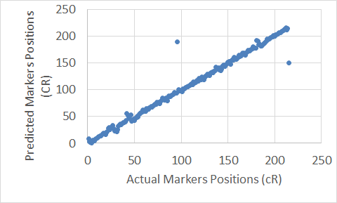Figure 7.  The Extended Clustering Method map for Chromosome 3.

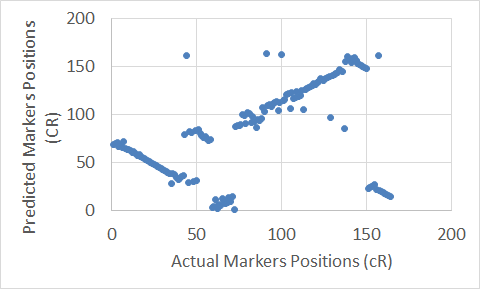Figure 8.  The Carthagene tool map for Chromosome 3.

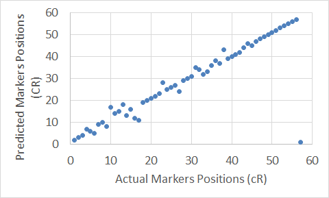Figure 9.  The Extended Clustering Method map for Chromosome 10.

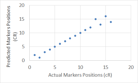Figure 10.  The Carthagene tool map for Chromosome 10.

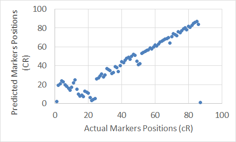Figure 11.  The Extended Clustering Method map for Chromosome 16.

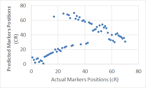Figure 12.  The Carthagene tool map for Chromosome 16.

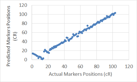Figure 13.  The Extended Clustering Method map for Chromosome 18.

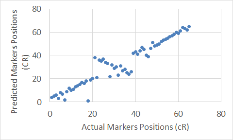Figure 14.  The Carthagene tool map for Chromosome 18.

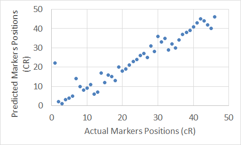Figure 15.  The Extended Clustering Method map for Chromosome 21.

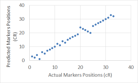Figure 16.  The Carthagene tool map for Chromosome 21.

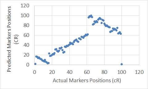Figure 17.  The Extended Clustering Method map for Chromosome 7.

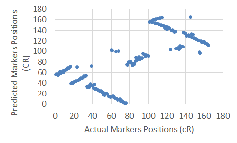Figure 18.  The Carthagene tool map for Chromosome 7.

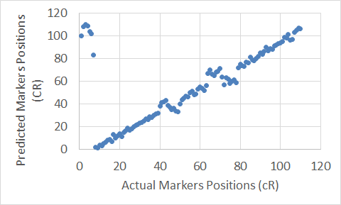Figure 19.  The Extended Clustering Method map for Chromosome 15.

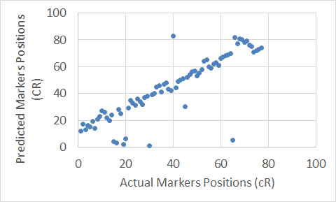Figure 20.  The Carthagene tool map for Chromosome 15.

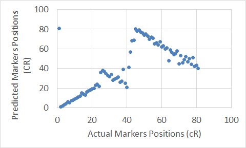Figure 21.  The Extended Clustering Method map for Chromosome 12.

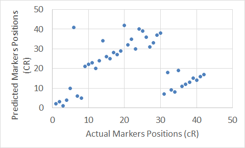Figure 22.  The Carthagene tool map for Chromosome 12.

1. Seetan, R.I., Bible, J., Karavias, M., Seitan, W. and Thangiah, S., 2016, December. Consensus Clustering: A Resampling-Based Method for Building Radiation Hybrid Maps. In Machine Learning and Applications (ICMLA), 2016 15th IEEE International Conference on (pp. 240-245). IEEE. doi: 10.1109/ICMLA.2016.0047
2. Kalavacharla V, Hossain K, Riera-Lizarazu O, Gu Y, Maan SS, Kianian SF. Radiation hybrid mapping in crop plants. Advances in agronomy. 2009 Dec 31;102:201-22. doi: 10.1016/s0065-2113(09)01006-2
3. Goss SJ, Harris H. New method for mapping genes in human chromosomes. Nature. 1975 Jun 26;255(5511):680-4. doi: 10.1038/255680a0
4. Seetan, R.I., Denton, A.M., Al-Azzam, O., Kumar, A., Iqbal, M.J. and Kianian, S.F., 2014. Reliable radiation hybrid maps: an efficient scalable clustering-based approach. IEEE/ACM Transactions on Computational Biology and Bioinformatics, 11(5), pp.788-800. doi: 10.1109/tcbb.2014.2329310
5. Ben-Dor A, Chor B, Pelleg D. RHO—radiation hybrid ordering. Genome Research. 2000 Mar 1;10(3):365-78. doi: 10.1101/gr.10.3.365
6. Press WH, Teukolsky SA, Vetterling WT, Flannery BP. Numerical Recipes in Fortran 77, The Art of Scientific Computing, 1992. doi: 10.5860/choice.30-5638a
7. Cvijovic D, Klinowski J. Taboo search: an approach to the multiple minima problem. Science. 1995 Feb 3;267(5198):664-6.
8. Helsgaun K. An effective implementation of the Lin–Kernighan traveling salesman heuristic. European Journal of Operational Research. 2000 Oct 1;126(1):106-30. doi: 10.1016/s0377-2217(99)00284-2
9. Seetan, R.I., Denton, A.M., Al-Azzam, O., Kumar, A., Iqbal, M.J. and Kianian, S.F., 2014, September. A noise-aware method for building radiation hybrid maps. In Proceedings of the 5th ACM Conference on Bioinformatics, Computational Biology, and Health Informatics (pp. 541-550). ACM. doi: 10.1145/2649387.2649443
10. SDM. 2014. Seetan, R.I., Denton, A.M., Al-Azzam, O., Kumar, A., Sturdivant, J. and Kianian, S.F., 2014, April. Iterative framework radiation hybrid mapping. In Proceedings of the 2014 SIAM International Conference on Data Mining (pp. 1028-1036). Society for Industrial and Applied Mathematics. doi: 10.1137/1.9781611973440.117
11. De Givry S, Bouchez M, Chabrier P, Milan D, Schiex T. CARHTA GENE: multipopulation integrated genetic and radiation hybrid mapping. Bioinformatics. 2004 Dec 14;21(8):1703-4. doi: 10.1093/bioinformatics/bti222
12. Stein L, Kruglyak L, Slonim D, Lander E. RHMAPPER, unpublished software. Whitehead Institute/MIT Center for Genome Research. 1995. doi: 10.1093/bioinformatics/14.6.538
13. Matise TC, Perlin M, Chakravarti A. Automated construction of genetic linkage maps using an expert system (MultiMap): a human genome linkage map. Nature genetics. 1994 Apr 1;6(4):384-90. doi: 10.1038/ng0494-384
14. Morton NE. Sequential tests for the detection of linkage. American journal of human genetics. 1955 Sep;7(3):277. doi: 10.1002/gepi.1370060402
15. Ronin Y, Mester D, Minkov D, Korol A. Building reliable genetic maps: different mapping strategies may result in different maps. Natural Science. 2010 Jun 30;2(06):576. doi: 10.4236/ns.2010.26073
16. Mester, D.I., Ronin, Y.I., Korostishevsky, M.A., Pikus, V.L., Glazman, A.E. and Korol, A.B., 2006. Multilocus consensus genetic maps (MCGM): formulation, algorithms, and results. Computational biology and chemistry, 30(1), pp.12-20. doi: 10.1002/gepi.1370030105
17. Chaubey YP. Resampling methods: A practical guide to data analysis. Springer, 2001. doi: 10.2307/1271090
18. Sneath PH, Sokal RR. Numerical taxonomy. The principles and practice of numerical classification. 1973. doi: 10.2307/2285473
19. Stewart EA, McKusick KB, Aggarwal A, Bajorek E, Brady S, Chu A, Fang N, Hadley D, Harris M, Hussain S, Lee R. An STS-based radiation hybrid map of the human genome. Genome research. 1997 May 1;7(5):422-33.
20. Lunetta KL, Boehnke M, Lange K, Cox DR. Selected locus and multiple panel models for radiation hybrid mapping. American journal of human genetics. 1996 Sep;59(3):717.
21. Gyapay G, Schmitt K, Fizames C, Jones H, Vega-Czarny N, Spillett D, Muselet D, Prud’Homme JF, Dib C, Auffray C, Morissette J. A radiation hybrid map of the human genome. Human Molecular Genetics. 1996 Mar 1;5(3):339-46. doi: 10.1093/hmg/5.3.339
22. Kinsella RJ, Kähäri A, Haider S, Zamora J, Proctor G, Spudich G, Almeida-King J, Staines D, Derwent P, Kerhornou A, Kersey P. Ensembl BioMarts: a hub for data retrieval across taxonomic space. Database. 2011 Jan 1;2011. doi: 10.1093/database/bar030
23. Amid C, Birney E, Bower L, Cerdeño-Tárraga A, Cheng Y, Cleland I, Faruque N, Gibson R, Goodgame N, Hunter C, Jang M. Major submissions tool developments at the European Nucleotide Archive. Nucleic acids research. 2011 Nov 12;40(D1):D43-7. doi: 10.1093/nar/gkr946
24. Kumar A, Seetan R, Mergoum M, Tiwari VK, Iqbal MJ, Wang Y, Al-Azzam O, Šimková H, Luo MC, Dvorak J, Gu YQ. Radiation hybrid maps of the D-genome of Aegilops tauschii and their application in sequence assembly of large and complex plant genomes. BMC genomics. 2015 Oct 16;16(1):800. doi: 10.1186/s12864-015-2030-2
25. Kumar A, Mantovani EE, Seetan R, Soltani A, Echeverry-Solarte M, Jain S, Simsek S, Doehlert D, Alamri MS, Elias EM, Kianian SF. Dissection of genetic factors underlying wheat kernel shape and size in an elite× nonadapted cross using a high density SNP linkage map. The plant genome. 2016 Mar 1;9(1). doi: 10.3835/plantgenome2015.09.0081

(Click to view)

(Click to view)