1. Introduction

Epilepsy in humans is an intrinsic brain pathology and its major manifestation is epileptic seizures. Epileptic seizures may affect partial part of the brain (partial) or the whole cerebral mass (generalized), seizures are recurrent with interictal period ranging from several minutes to several days. Brain’s electrical activity is measured through the electroencephalogram (EEG) signal which is an effective tool for studying functioning of brain and diagnosing epilepsy [1]. EEG signals are a non-invasive testing method that provides valuable details of distinct physiological states of the brain. The data recorded usually are of long duration and inspected by experts to analyze the huge data recorded in the form of EEG signal to detect epilepsy.

The advanced signal processing has enabled to process and store the EEG signal digitally. The proThe automatic system reduces the workload of neurologists by reducing the amount of effort and time required to detect the traces of epilepsy in the recorded EEG signal. Automatic prediction and detection of epilepsy from the EEG signal are developed using different signal processing techniques like frequency domain analysis, wavelet analysis, spike detection, and non-linear methods. Gotman [2] has presented an automatic detection system for epilepsy by decomposing the EEG signal into elementary waves. Srinivasan et al., [3] has used time domain and frequency domain analysis to detect epilepsy the author has selected five features out of which two features were from frequency-domain and three features were from time-domain. The author has used the recurrent neural network for detecting epilepsy and the neural net-

work was trained and tested for the epileptic EEG signal with an accuracy of 99.6%, Keshri et al., [4] has used the slope of the lines between each pair of two consecutive data points (x1, y1) and (x2, y2) and feed it into Deterministic Finite Automata and got the accuracy level as high as 95.68%. Geva et al., [5] has used wavelet analysis as both time and frequency domain view can be provided with the use of WT.

Various methods are available to detect and predict the epileptic seizure. Artificial Neural Network (ANN) has been widely used for detecting the epileptic spike [1, 6, 7, 8, 9]. Features extraction is an important aspect in the performance of ANN models as the model is trained in and tested on these extracted features. ApEn was proposed by Pincus [10] as a statistical parameter to measure the regularity of time series data. ApEn is being predominantly used in the electrocardiogram and other related heart rate data analysis [11, 12, 13] as well as in the analysis of endocrine hormone [14]. It is the measure of regularity as smaller value of ApEn depicts a high regularity and higher value of ApEn depicts low regularity in time series data [15]. Diambra et al., [16] has denoted that parameter ApEn gives the valuable temporal localization of a variety of epileptic activity. Elman, PNN and SVM network for detection of epilepsy through ApEn based feature with 100% overall accuracy. Hence, it is an acceptable feature for automated detection of epilepsy.

The Support Vector Machine (SVM) is a classier method that performs classification tasks by constructing hyperplanes in a multidimensional space which try to find a combination of samples to build a plane maximizing the margin between two classes. SVM is widely used in epileptic detection and prediction [17] has used permutation entropy as a parameter, as it drops during the seizure interval. The Burg Burg AR coefficients has been used as an input for SVM that shows accuracy of 99.56% [18].

In this paper an automated detection of the epileptic seizure was discussed using LS-SVM comparing two kernel functions RBF and linear. In this work EEG signal were decomposed into six sub-bands namely D1-D5 and A5 using DWT. The analysis of complexity in the sub-bands are done by ApEn which acts as an input feature for SVM. Experiments are done using different cases having a different combination of EEG data sets.

2.      Proposed Method

In this paper there are four main tasks in sections 2.1) Clinical data 2.2) Preprocessing EEG data through DWT to decompose into several sub-bands in section 2.3) Feature extraction (ApEn) in section 2.4 ) Classification of EEG data using feature (ApEn). Figure 1 shows the proposed approach used in this paper.

2.1. Clinical data

The data set used in this paper is available in public domain and is accessed online from the University of Bonn, Germany which consists of five different data set of EEG data [19]. The data used is artifact free EEG time series data and is widespreadly used by the ongoing research on epilepsy [1, 3, 7, 15, 17, 20]. The complete data set contains five sets marked as (A-E) each set has 100 single channel EEG segment having duration of 23.6-sec. Each segments of data are selected and cut out after visual inspection for artifacts from continuous mechanical EEG recordings with the sampling frequency of 173.61 Hz with the band pass settings of 0.53-40 Hz. The data contains three different classes normal, epileptic background (pre-ictal), and epileptic seizure (ictal). The normal EEG data (A and B) was collected from five healthy volunteers. The pre-ictal EEG data (C and D) was recorded during the period when there were no traces of seizure from five epileptic patients. The ictal EEG data (E) was recorded during the epileptic seizure from the same five patients. EEG signals were recorded from 128- channel amplifier using an average common reference and digitized at 173.61 Hz sampling rate and 12-bit A/D resolution. Figure 2 and Figure 3 shows the specimen of an epileptic and normal signal.

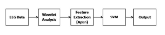Figure 1. Proposed Approach

2.2. Discrete Wavelet Transform

Wavelet transform (WT) uses variable window size, has well-known data compression and timefrequency filtering capabilities. It provides a good local representation of the signal in time as well as in the frequency domain which makes it as an effective tool for analyzing the signal and extracting features. The wavelet transform looks for the spatial distribution of singularities whereas fourier transform provides a description of the overall regularity of signals [5].

WT captures transient features and localizes them in time as well as frequency content and is widely used in epileptic seizure detection [21, 22]. WT uses long time windows for obtaining finer low-frequency resolution as well as the short time windows for obtaining high-frequency information. Thus, WT provides specific frequency information at low frequencies and specific time information at high frequencies [23].

Discrete wavelet transform (DWT) x(t), is defined

as,

                                              1 Z ∞                         t − 2^jk!

              DWT                                    x(t)ψ     dt         (1)

2j

Where ψ, a and b are wavelet function called as scaling and shifting parameters. The quadrature mirror filters are used to realize the scheme by passing the passing the signal through a series of low-pass (LP) and high-pass (HP) filter [24] The out put from the low pass filter is termed as . Approximation (A) and output from the high pass filter id termed as detail (D) coefficients. The figure illustrates the fifth level wavelet decomposition of a signal showing the coefficients A1, D1, A2, D2, A3, D3, A4, D4, A5, and D5

.

In this model fifth-level wavelet decomposition was performed on normal subjects data (A, B, C and D) as well as on epileptic patient data (E) using Daubechies order 4 wavelet (db4). The researchers have found that db4 wavelet is most appropriate for the analysis of epileptic EEG data [25]. The structure for the wavelet decomposition at each level with its approximation and detail coefficients are shown in Figure 4.

2.3. Approximate entropy (ApEn)

Approximate entropy is a statistical feature for quantifying regularity and complexity in a time-series data [10]. ApEn is a non-negative number and has been successfully applied in the field of pattern recognition. ApEn have potential application throughout medicine and prominently in ECG and EEG [14].The following steps determine the value of ApEn [1, 8, 26, 27, 28].

1. The data set contains N data points let it beA=[a(1), a(2), . . . , a(N-m+1)].
2. Let a(i) be a subsequence of A such that a(i) =[a(i), a(i+1), a(i+2), . . . , a(i+m-1)] for 1 ≤ i ≤ N − m+1, m is the number of samples used
3. Denote the distance between A(i) and A(j) byd[A(i), A(j)]=

max      (| a(i +1) − a(j +1) |)            (2) k=0,…,m−1

4. For a given A(i), number of j is counted as (j = 1,…,N − m + 1,j , i) such that d[A(i),A(j)] ≤ r denoted as M^m(i) for i = N − m+1

                                          m                        Mm(i)

                                Cr (i) = (N − m+1),               (3)

for i = 1,…,N − m+1

5. For each C_r^m(i) compute natural logarithm, and average it over i

N−m+1

Φ^m(r) =    −¹m+1 ^X lnC_r^m(i)     (4) N

i=1

6. . Repeat step (1) to step (4) by increasing the dimension m to m+1 and find C_r^m+1(i) and Φ^m+1(r)
7. Finally ApEn is computed as

                               ApEn(m,r,N) = Φ^m(r) − Φ^m+1(r)               (5)

To compute the ApEn value of the signal of length N two parameters length of the compared run m tolerance window r are specified. We have taken the value of m=2 and 3 and r is in between 0.1 to 0.25 times the standard deviation of data. In this model the ApEn values of the approximate (A1-A5) and detailed coefficients (D1-D5) are computed using the length of the compared run (m), tolerance window (r) were set to m= (2,3) and r= (0.2)*standard deviation of the data to compute ApEn.

2.4. Support vector machine (SVM)

Support vector machine (SVM) has been used in several EEG signal classification problems [17, 20] and was first introduced in 1995. SVMs belong to the family of kernel-based classifiers and are extremely powerful classifiers. Linear as well as non-linear classification can be performed in SVM using different kernel functions [29]. The approach of SVMs is to implicitly map the classification data into higher dimension input space where a hyperplane separating the classes may exist. The implicit mapping is achieved through different Kernel functions. In the case of linear SVM to classify linearly separable data, the training data, {a_i,b_i} for i = 1,,m and y_i ∈ {−1,1} then the following decision function is determined by [18]:

                                      D (x) = w^tg(x)+y                                  (6)

g(x)is a mapping function that maps x into ldimensional space, y is a scalar and w is the ldimensional vector. The decision function satisfies the following condition to separate the data linearly:

                     b_i w^tg      f or      i = 1,,M               (7)

i           i                       ≥ ρ          f or   i = 1,,M kwk The product of ρ and kwkis fixed	(8)
ρkwk = 1	(9)

There are infinite number of decision functions that satisfy Eq.(8) for a linearly separable feature space. The largest between the two classes are selected between the two classes. The margin given by D |x|/ kwk. Let the margin is ρ then the following condition are required to be satisfied: ^{b D (a )}

In order to obtain the maximum margin for the optimal separating hyperplane, w¯ with the minimum kwk that satisfying Eq. (9) should be found from Eq. (10), This provides optimization problem as follows. Minimizing

• ^tw (10) w
• subject to            the          constraints:           b_i w^tg (a_i)+y ≥ 1     f or          i = 1,,M When training data are not linearly separable a slack variables is introduced ξ_i into

Eq. (8)

b_i w^tg           f or         i = 1,,M (11)

To maximize the margin and minimize the training error the optimal separating hyperplane is determined and is achieved by minimizing,

n

21       tw + C2 Xξip                  (12) w

i=1

subject to the constraints:b_i w^tg (a_i)+b ≥ 1 − ξ_i, ξ_i ≥ 0 f or i = 1,,M

The tradeoff between the maximum margin and minimum classification error is determined by the parameter C.

2.5. Least squares support vector machines (LS-SVMs)

The LS-SVM are trained by minimizing

n

                                   12wtw + C2 Xξi2                                         (13)

i=1

subject to the equality constraints:

b_i w^tg (a_i)+y = 1−ξ_i,                    ξ_i ≥ 0      f or         i = 1,,M (14)

The conventional SVM uses inequality constraints where as in the LS-SVM equality constraints are used. The equality constraint has reduced the complexity to obtain the optimal solution by solving a set of linear equations rather than solving a quadratic programming problem. To derive the dual problem of Eqs.

(14) and (15) Lagrange multipliers are used

Q(w,y,α,ξ)

                              n                    M

• tw + C Xξi2 − Xαi nyi wtg (ai)+y − 1+ξio

=         w

• 2

                             i=1                  i=1

(15)

where α = (α_i,…,α_M)^t is Lagrange multipliers and by differentiating the above equation with respect to w,ξ_i,b, and α_i and equating the resulting equations to zero the the conditions for optimality are determined

[30].

2.5.1. Kernel Function

Classically SVMs were designed to classify the data in linear space, in the nonlinear space SVMs do not preformed well to overcome this limitation on SVMs, kernel approaches were developed. The following kernels are most commonly used [31].

1. Linear Kernels: k(a,a⁰ ) = (a^ta⁰ );
2. Polynomial kernels: k(a,a⁰ ) = ((a^ta⁰ ) + 1)^y where d is a positive intege r
3. RBF kernels: ka,a0 = exp−γ    a − a0

To train a SVM classifier, the user has to determine a suitable kernel function, optimum hyper parameters, and proper regularization parameter. in this paper we have used two kernels 1) Linear Kernel and 2) RBF kernel. The goal to achieve optimum hyper parameter and regularization parameter is accomplished by cross-validation technique. The crossvalidation technique can be used to select parameters.

2.6. Cross-Validation

Cross-validation is a validation technique used to determine the quality of the classification model. It partitions a sample data into different subsets such that the analysis is initially implemented on a single subset. The remaining subset(s) are kept for validating the result of initial analysis. The data subset used for initial test is called as training set while the other subsets are called as testing or validation sets [32]. In K-Fold cross validation data is partitioned into k roughly equal size sets and each set is used once as a test set while other remaining sets are used as training sets. For each k=1,2,…N, fit the model parameter for other retained K-1 parts. The cross-validation procedure is repeated for K number of times using each of the K set exactly once as validation data. The average of the K result obtained from the folds produces a single estimation. In this paper, we have used 10-fold scheme to achieve best performance efficiency.

2.7. Performance evaluation parameters

The performance of LS-SVM is estimated by using the parametres, namely, sensitivity (SE), specificity (SP) and overall accuracy (OA) defined as:

                                                    T N^CP ∗ 100                          (16)

SE(%) = T N_AP

Where T N_CP denotes the count of correctly detected positive patterns and T N_AN denotes the count of actual positive pattern. The positive pattern represents a detected seizure.

                                                    T N^CN ∗ 100                          (17)

SP (%) =

T N_AN

Where T N_CN denotes the count of correctly detected negative pattern and T N_AN denotes the actual count of negative pattern. The negative pattern represents a detected non-seizure.

                                                   T N^CDP ∗ 100                         (18)

OA(%) = T NAP P

Where T N_CDP denotes the count of correctly detected pattern and T N_{AP P} denotes the count of applied patterns [1].

3.    Design of Experiment

The data is processed and the ApEn values of the detailed and approximate coefficients are computed. The design of experiment is done to make different cases of the processed data-set and then compare the results of different cases the cases are as follows

• Case 1: Data set A versus Data set E
• Case 2: Data set B versus Data set E
• Case 3: Data set C versus Data set E
• Case 4: Data set D versus Data set E
• Case 5: Data set A, C and D versus Data set E
• Case 6: Data set A, B, C and D versus Data set E

These cases are then modeled combining all the coefficients A5 and D1-D5 in one set as an input to LSSVM and using different coefficients individually as an input to LS-SVM. The results were analyzed using all different cases and combinations and compared to find the model providing the best efficiency.

4.    Result and Discussion

The EEG data set is decomposed into different sub bands by applying DWT using db4 wavelet having 5 level of decomposition shown in Figure 4. The frequency ranges of these sub-bands are: A1(043.4 Hz), A2 (021.7Hz), A3 (010.85Hz), A4 (05.43 Hz),

A5 (02.70Hz), D1 (43.486.8 Hz), D2 (21.743.4 Hz),

D3 (10.8521.7Hz), D4(5.4310.85Hz) and D5 (2.705.43 Hz. ApEn values have been computed from the approximation and detail coefficients of each sub-bands of entire 500 EEG epochs of five data sets A-E. Figure 5 and 6 shows the decomposition of EEG signal epoch of data set A and E.

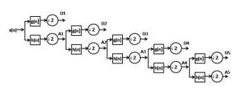Figure 4. Decomposition of EEG signal using fifth level decomposition

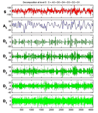Figure 5. WaveletdecompositionofEpilepticsignal(DataSet E)

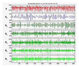Figure 6. Wavelet decomposition of Normal Signal (Data Set A )

is used to train the SVM while testing data set is used for verifying the accuracy of the trained SVM. For dividing the data set into training and testing part we have used holdout method of cross validation. The SVM is initialized by initlssvm function trained using tunelssvm and trainlssvm function. The performance parameters were tuned by using tunelssvm function for regularization and kernel parameter (gam, sig2) of LS-SVM [34]. The SVM algorithm is used with linear and Gaussian radial basis kernel functions. Linear kernel function require gamma parameter for training the SVM. SVM with rbf kernel function require gamma as well as sigma parameter which has to be selected based on training data. In this paper we have set gamma ∈ [0 − 1] for linear Kernel and gamma ∈ [0 − 10] for

The ApEn values of the approximate and detailed coefficients are computed from the entire data set AE consisting 100 epochs having parameters m=(2,3) and r=0.2*standard deviation of data set. ApEn value of the detailed coefficient D1 from data set A, B which were recorded from the surface of the scalp of the normal subject while they are in a relaxed and an awake state with (Data Set A) eyes open and (Data set B) eyes closed vs E are recorded from the epileptic subjects through intracranial electrodes and having embedded Figure 8. Normal Signal

In this paper SVM is implemented by using MATLAB R2012b and LS-SVM toolbox [33].The input feature vector ApEn is divided into two parts training data set 60% and testing 40%. The training data set rbf Kernel. The sigma parameter for rbf kernel is ∈ [0.7 − 9] using tunelssvm function. Each row of the input data matrix is one observation and its column is one feature.

Table 1. Statistical parameters with ApEn embedded dimension m=2 linear kernel Embedding dimension (m=2) SVM (Linear)         Cases for seizure detection D1 D2 D3 D4 D5 A5 Case 1 (A-E) 0.9875 0.9375 0.9375 0.8625 0.55 0.95 Case 2 (B-E) 0.9375 0.9375 0.7375 0.7625 0.575 0.9125 Case 3 (C-E) 0.9875 0.975 0.875 0.6375 0.775 0.8625 Case 4 (D-E) 0.95 0.7875 0.7 0.5875 0.7625 0.825 Case 5 (ACD-E) 0.925 0.8875 0.8063 0.7562 0.7813 0.9063 Case 6 (ABCD-E) 0.94 0.89 0.83 0.81 0.805 0.925 Table 2. Statistical parameters with ApEn embedded dimention m=2 rbf Embedding dimension (m=2) SVM (RBF)         Cases for seizure detection D1 D2 D3 D4 D5 A5 Case 1 (A-E) 0.9875 0.95 0.975 0.875 0.5875 0.9 Case 2 (B-E) 0.9625 0.9375 0.75 0.7875 0.6 0.9 Case 3 (C-E) 0.9875 0.9625 0.925 0.675 0.85 0.875 Case 4 (D-E) 0.925 0.75 0.7375 0.5875 0.825 0.875 Case 5 (ACD-E) 0.9437 0.9125 0.825 0.7688 0.8063 0.9063 Case 6 (ABCD-E) 0.945 0.91 0.84 0.84 0.815 0.93

The feature vector of each data set has 100 rows (epochs) and 6 columns (D1-D5) and A5. Case (1 − 4) consist 200 observations, Case 5 consist of 400 observations, Case 6 consists 500 observations. The observations are normalized by scaling between 0 and 1 and then 60% and training and 40% of testing data is used for training and testing SVM.

Fig.7: The Case when D1-D5 and A5 is used individu-ally as an Input to LS-SVM

The highest precision accuracy of for embedded dimension m = 2 are found in cases 1 and 3 for detailed coefficient D1 are 98.75% using linear kernel and same for rbf kernel ie. in cases 1 and 3 are 98.75%. The lowest accuracy was found to be 55% for case 1 for detailed coefficient D5 in linear kernel and 59% for case 1 for detailed coefficient D5 in rbf kernel. The results suggests that there is marginal differences between the results of rbf and linear kernel but the overall average efficiency remains same for both in this cases as shown in the Table 1 and Table 2. The highest accuracy of for embedded dimension m = 3 is found in cases 1,2 and 3 for detailed coefficient D1 are 96.25% and for RBF kernel it is 98.75% for cases 1 and 3 for detailed coefficient D1. In this modeling RBF kernel shows better results than that of linear kernel the overall result is summarized in Table 3 and Table

4.

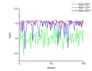Fig.8: The Case when D1-D5 and A5 is combined as anInput to LS-SVM

The precision of the proposed system for embedded dimension m = 2 with linear kernel is 100% which is maximum and a lowest of 98:12% respectively for cases 1, 3, 4, 5 and case 6. Similarly, the precision of the proposed system for embedded dimension m = 2 with RBF kernel is 100% maximum and lowest of 99.50% respectively for cases 1-5 and case 6. The precision of the proposed system for embedded dimension m = 3 with linear kernel is 100% maximum and a lowest of 97.0% respectively for cases 1, 3, 4 and case 6. Similarly, the precision of the proposed system for embedded dimension m = 3 with RBF kernel is 100% maximum and a lowest of 99.5% respectively for cases 1, 3 − 5 and case 6. It is clearly observed in the results summarized in Table 6 and Table 7 that RBF kernel based automatic epileptic seizure detection system gives better precision than linear kernel based automatic epileptic seizure detection system. Table 5 presents the the comparison of results between the existing and the proposed method using same data set.

5.    Conclusion and Future Scope

The least squares version of support vector machine classifiers is discussed in this paper. The quadratic programming problem has been eased to solving a set of linear equations with the use of equality constraint instead of inequality constraint. In this paper we have modeled LS-SVM using EEG data set with different combinations of input features as well as changing the parameters of the ApEn. The results suggest that the combination of detailed and approximate coefficients ie. D1-D5 and A5 as an input to classifier produces better results than using single feature D1 as a classification input. The kernel function also plays significant role in the classifying the EEG data set using LS-SVM and RBF kernel produces better results than the linear kernel in this modelling. The embedded dimension m for calculation the ApEn is also significant ad this model suggests that at m=2 the classification system performs better than that at m=3. The proposed approach can be deployed as a quantitative measure for monitoring EEG signal associated with epilepsy. As an extension of the proposed method, it would be challenging to scrutinize the efficacy of the proposed method for other neurological disorders which uses brain signals for analyzes such as Parkinson diseases etc [35]. Furthermore, it would be interesting to analyze the learning effectiveness of this model on other database. In this study, the

Embedding dimension (m=2)	SVM (Linear)			SVM (RBF)
Cases for seizure detection	SE	SP	OA	SE	SP	OA
Case 1 (A-E)	1	1	1	1	1	1
Case 2 (B-E)	0.9722	1	0.9875	1	1	1
Case 3 (C-E)	1	1	1	1	1	1
Case 4 (D-E)	1	1	1	1	1	1
Case 5 (ACD-E)	1	0.9831	0.9875	1	1	1
Case 6 (ABCD-E)	0.9697	0.982	0.98	0.9756	1	0.995

Table 3. Statistical parameters with ApEn embedded dimention m=3 lin

Embedding dimension (m=3)	SVM (Linear)
Cases for seizure detection	D1	D2	D3	D4	D5	A5
Case 1 (A-E)	0.9625	0.9375	0.95	0.9875	0.7125	0.925
Case 2 (B-E)	0.9625	0.8875	0.775	0.7125	0.7375	0.875
Case 3 (C-E)	0.9625	0.95	0.8625	0.8	0.6375	0.875
Case 4 (D-E)	0.9125	0.8	0.7	0.7125	0.6	0.7625
Case 5 (ACD-E)	0.9	0.85	0.8	0.775	0.8063	0.875
Case 6 (ABCD-E)	0.905	0.885	0.85	0.83	0.84	0.895
Table 4. Statistical par	ameters wit	h ApEn em	bedded dim	ention m=3	rbf
Embedding dimension (m=3)	SVM (RBF)
Cases for seizure detection	D1	D2	D3	D4	D5	A5
Case 1 (A-E)	0.9875	0.9375	0.9375	0.9875	0.7	0.925
Case 2 (B-E)	0.975	0.925	0.825	0.7875	0.7375	0.85
Case 3 (C-E)	0.9875	0.9625	0.875	0.8125	0.65	0.875
Case 4 (D-E)	0.9125	0.825	0.775	0.7375	0.65	0.7875
Case 5 (ACD-E)	0.9437	0.885	0.85	0.8438	0.8187	0.8938
Case 6 (ABCD-E)	0.95	0.91	0.85	0.83	0.845	0.895

Table 5. Comparison with Existing Models

Authors	Year	Method	Cases	Maximum OA %
Srinivasan et al. [3]	2005	Time and frequency domain features using ANN	Case 1	99.60
Srinivasan et al. [1]	2007	Approximate Entropy using ANN	Case 1	100
Ocak [7]	2009	DWT and (ApEn)	Case 1 Case 9	99.60 96.65
Guo et al. [8]	2010	Discrete wavelet transform using ANN	Case 1 Case 9	99.85 98.27
Ubeyli [18]	2010	LS-SVM model-based method coefficients	Case 1	99.56
Nicolaou et al [17]	2012	Permutation entropy using SVM	Case 1 Case 2 Case 3 Case 4	93.55 82.88 88.00 79.94
Kai et al. [36]	2014	Time-frequency image using SVM	Case 1	99.125
Anindya et al. [37]	2016	Dual tree complex wavelet transform using SVM	Case 1 Case 3 Case 4 Case 9	100 100 100 100
Proposed Method		DWT based ApEn and Artificial neural network, LS-SVM	Case1 Case2 Case3 Case4 Case5 Case6	100 100 100 100 100 99.5

Table 6. Results obtained for proposed model with embedded dimension m=2 Table 7. Results obtained for proposed model with embedded dimension m=3

Embedding dimension (m=2)	SVM (Linear)			SVM (RBF)
Cases for seizure detection	SE	SP	OA	SE	SP	OA
Case 1 (A-E)	1	1	1	1	1	1
Case 2 (B-E)	0.9474	1	0.975	0.975	1	0.9875
Case 3 (C-E)	1	1	1	1	1	1
Case 4 (D-E)	1	1	1	1	1	1
Case 5 (ACD-E)	0.9524	0.9915	0.9812	1	1	1
Case 6 (ABCD-E)	0.9091	0.982	0.97	0.995	0.9939	0.995

proposed model has been tested on different datasets from the same database.

1. V. Srinivasan, C. Eswaran, N. Sriraam, Approximate entropybased epileptic eeg detection using artificial neural networks, Information Technology in Biomedicine, IEEE Transactions on 11 (3) (2007) 288–295.
2. J. Gotman, Automatic recognition of epileptic seizures in the eeg, Electroencephalography and clinical Neurophysiology 54 (5) (1982) 530–540.
3. V. Srinivasan, C. Eswaran, Sriraam, N, Artificial neural network based epileptic detection using time-domain and frequency-domain features, Journal of Medical Systems 29 (6) (2005) 647–660.
4. A. K. Keshri, R. K. Sinha, R. Hatwal, B. N. Das, Epileptic spike recognition in electroencephalogram using deterministic finite automata, Journal of medical systems 33 (3) (2009) 173–179.
5. A. B. Geva, D. H. Kerem, Forecasting generalized epileptic seizures from the eeg signal by wavelet analysis and dynamic unsupervised fuzzy clustering, Biomedical Engineering, IEEE Transactions on 45 (10) (1998) 1205–1216.
6. A. Alkan, E. Koklukaya, A. Subasi, Automatic seizure detection in eeg using logistic regression and artificial neural network, Journal of Neuroscience Methods 148 (2) (2005) 167–176.
7. H. Ocak, Automatic detection of epileptic seizures in eeg using discrete wavelet transform and approximate entropy, Expert Systems with Applications 36 (2) (2009) 2027–2036.
8. L. Guo, D. Rivero, A. Pazos, Epileptic seizure detection using multiwavelet transform based approximate entropy and artificial neural networks, Journal of neuroscience methods 193 (1) (2010) 156–163.
9. A. Subasi, J. Kevric, M. A. Canbaz, Epileptic seizure detection using hybrid machine learning methods, Neural Computing and Applications (2017) 19.
10. S. M. Pincus, Approximate entropy as a measure of system complexity., Proceedings of the National Academy of Sciences 88 (6) (1991) 2297–2301.
11. K.-J. Bar, M. K. Boettger, M. Koschke, S. Schulz, P. Chokka,  V. K. Yeragani, A. Voss, Non-linear complexity measures of heart rate variability in acute schizophrenia, Clinical Neurophysiology 118 (9) (2007) 2009–2015.
12. K. K. Ho, G. B. Moody, C.-K. Peng, J. E. Mietus, M. G. Larson, D. Levy, A. L. Goldberger, Predicting survival in heart failure case and control subjects by use of fully automated methods for deriving nonlinear and conventional indices of heart rate dynamics, Circulation 96 (3) (1997) 842–848.
13. X. Hu, C. Miller, P. Vespa, M. Bergsneider, Adaptive computation of approximate entropy and its application in integrative analysis of irregularity of heart rate variability and intracranial pressure signals, Medical engineering & physics 30 (5) (2008) 631–639.
14. S. M. Pincus, I. M. Gladstone, R. A. Ehrenkranz, A regularity statistic for medical data analysis, Journal of clinical monitoring 7 (4) (1991) 335–345.
15. U. R. Acharya, F. Molinari, S. V. Sree, S. Chattopadhyay, K.-H. Ng, J. S. Suri, Automated diagnosis of epileptic eeg using entropies, Biomedical Signal Processing and Control 7 (4) (2012) 401–408.
16. L. Diambra, J. de Figueiredo, C. P. Malta, Epileptic activity recognition in eeg recording, Physica A: Statistical Mechanics and its Applications 273 (3 (1999) 495–505.
17. N. Nicolaou, J. Georgiou, Detection of epileptic electroencephalogram based on permutation entropy and support vector machines, Expert Systems with Applications 39 (1) (2012) 202–209.
18. E. D. Ubeyli, Least squares support vector machine employing model-based methods coefficients for analysis of eeg signals, Expert Systems with Applications 37 (1) (2010) 233–239.
19. R. G. Andrzejak, K. Lehnertz, F. Mormann, C. Rieke, P. David, C. E. Elger, Indications of nonlinear deterministic and finite-dimensional structures in time series of brain electrical activity: Dependence on recording region and brain state, Physical Review E 64 (6) (2001) 061907.
20. Y. Kumar, M. L. Dewal, R. S. Anand, Relative wavelet energy and wavelet entropy based epileptic brain signals classification, Biomedical Engineering Letters 2 (3) (2012) 147–157.
21. A. Subasi, E. Erc¸elebi, Classification of eeg signals using neural network and logistic regression, Computer methods and programs in biomedicine 78 (2) (2005) 87–99.
22. S. Patidar, T. Panigrahi, Detection of epileptic seizure using kraskov entropy applied on tunable-q wavelet transform of eeg signals, Biomedical Signal Processing and Control 34 (2017) 74–80.
23. H. Ocak, Optimal classification of epileptic seizures in eeg using wavelet analysis and genetic algorithm, Signal processing 88 (7) (2008) 1858–1867.
24. S. G. Mallat, A theory for multiresolution signal decomposition: the wavelet representation, Pattern Analysis and Machine Intelligence, IEEE Transactions on 11 (7) (1989) 674–693.
25. H. Adeli, Z. Zhou, N. Dadmehr, Analysis of eeg records in an epileptic patient using wavelet transform, Journal of neuroscience methods 123 (1) (2003) 69–87.
26. J. Bruhn, H. Ropcke, A. Hoeft, Approximate entropy as an electroencephalographic measure of anesthetic drug effect during desflurane anesthesia, Anesthesiology 92 (3) (2000) 715–726.
27. J. S. Richman, J. R. Moorman, Physiological time-series analysis using approximate entropy and sample entropy, American Journal of Physiology Heart and Circulatory Physiology 278 (6) (2000) H2039–H2049.
28. P. Artameeyanant, W. Chiracharit, K. Chamnongthai, Spike and epileptic seizure detection using wavelet packet transform based on approximate entropy and energy with artificial neural network, in: Biomedical Engineering International Conference (BMEiCON), 2012, IEEE, 2012, pp. 1–5.
29. C. J. Burges, A tutorial on support vector machines for pattern recognition, Data mining and knowledge discovery 2 (2) (1998) 121–167.
30. D. Tsujinishi, S. Abe, Fuzzy least squares support vector machines for multiclass problems, Neural Networks 16 (5) (2003) 785–792.
31. K. Polat, B. Akdemir, S. Gunes¸, Computer aided diagnosis of ecg data on the least square support vector machine, Digital Signal Processing 18 (1) (2008) 25–32.
32. T. Kayikcioglu, O. Aydemir, A polynomial fitting and¡ i¿ k¡/i¿-nn based approach for improving classification of motor imagery bci data, Pattern Recognition Letters 31 (11) (2010) 1207–1215.
33. J. A. Suykens, T. Van Gestel, J. De Brabanter, B. De Moor, J. Vandewalle, J. Suykens, T. Van Gestel, Least squares support vector machines, Vol. 4, World Scientific, 2002.
34. K. De Brabanter, P. Karsmakers, F. Ojeda, C. Alzate, J. De Brabanter, K. Pelckmans, B. De Moor, J. Vandewalle, J. Suykens, Ls-svmlab toolbox users guide, ESAT-SISTA Technical Report (2011) 10–146.
35. M. Nilashi, O. Ibrahim, A. Ahani, Accuracy improvement for predicting parkinsons disease progression, Scientific reports 6.
36. K. Fu, J. Qu, Y. Chai, Y. Dong, Classification of seizure based on the time-frequency image of eeg signals using hht and svm, Biomedical Signal Processing and Control 13 (2014) 15–22.
37. A. B. Das, M. I. H. Bhuiyan, S. S. Alam, Classification of eeg signals using normal inverse gaussian parameters in the dualtree complex wavelet transform domain for seizure detection, Signal, Image and Video Processing 10 (2) (2016) 259–266.

(Click to view)

(Click to view)