1          Introduction

Contractual agreements over prospective commodity flows already were established in the ancient. The commitment of transanctions to a fixed maturity reliably enabled long-term planning and reduced risks. The standardization of these so-called forwards to exchange-traded futures therefore only has been a question of time. Accordingly, futures have quickly spread after their first release at the Chicago Board of Trade in the 1860s. Modern futures markets offer high volumes and attractive trading conditions for numerous assets. This situation generates a highly interesting trading environment for speculative investors.

This paper is an extension of work originally presented in SSCI 2016 [1] in which different contract selection strategies have been introduced and tested in commodity markets. This research deepens the findings and improves the presented algorithm by refining the selection process. For this purpose, the new algorithm separates the ask and bid price structure to furtherly improve a case-dependent trading cost analysis. The results are evaluated by Monte Carlo simulations on sets of arbitrary trading instructions on three future classes in both, commodity and index futures. The analysis is settled on a broad fundament of historical data that enables a wider range of benchmarks than the previous paper. The results allow the conclusion of market inefficiencies in the analyzed markets.

     ⁶⁵                                                                                                            Maturity

2015−10−19

60

2015−12−18

     55                                                                                                                           2016−02−19

50

45

40

                    2015−07−01                                2015−09−01 2015−11−01

Maturity

16000                                                                                                                           2016−08−10

2016−09−08

2016−10−13 15000

14000

13000

2016−07−01 2016−09−01 2016−11−01

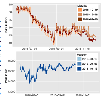Figure 1: Prices of three WTI future contracts (top chart) and three Nikkei future (bottom chart) contracts with different maturities

Among other properties, every future class is defined by a fix maturity interval in which corresponding contracts expire (typically one or three months). The life span of a contract however is an issue of supply and demand and generally considerably longer. Consequently, there are several coexistent contracts with different price structures and liquidities – all for

the same asset, but with different maturities. Due to individual risks and demand changes, different underlyings may exhibit significant disparities in their term structure properties. While consumer goods futures like natural gas show strong seasonal fluctuations, differences of index futures tend to more constant deviations [2]. Figure 1 exemplarily shows quotes for different WTI future contracts during the period from June to December 2016.

The application of conventional trading strategies in futures markets mandatorily generates the challenge of defining a strategy for the contract selection. As advantageous properties of a contract systematically result in other properties being unfavorable, the selection is always a nontrivial compromise with the objective of the best possible balance.

Of course, the prices of future contracts are significantly influenced by the current price of the underlying asset. However, an adequate model requires several additional factors to be taken into consideration. The definition of a formal relationship between future and spot price has been researched precisely and several models have been proposed [3–5]. The cost-of-carry model explains the price F_t,τ of a future contract with maturity τ at time t as a function of the spot price S given by

                                   F_t,τ = S_t · e(r+s−c)·(τ−t).                               (1)

The interest rate is divided into three parts: the risk-free interest rate r and storage cost s. Arising inaccuracies are explained by the so-called convenience yield c that covers all movements that are created by changing market expectations. Thereby, market situations like contango and backwardation can be constituted.

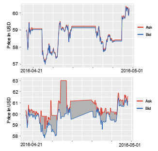Figure 2: Ask and bid quotes from two WTI Mini contracts with maturities July (above) and September (below) 2016 show huge differences in market liquidity and estimated trading costs

Figure 4 shows ask and bid quotes for two WTI Mini future contracts with maturities July and September 2016 during April 2016. Obviously, the spread highly depends on the time left to the maturity. The lower and much more persistent spread of the near contract yields favorable conditions. The notably smaller liquidility of contract markets with a more distant maturity generates an averagely higher spread. As the trading volume tremendously rises with a decreasing time span to the maturity, spreads tend to be the lowest for the nearest future contracts. While commissions follow a plain pattern, spreads between ask and bid prices strongly depend on market capitalization.

However, the acquisition of contracts with shortterm maturities for long-running positions require an extension of the expiry by re-opening positions for the same underlying asset. This procedure is called future rolling and results in additional trades and accordingly trading costs.

So, a suitable future contract selection strategy for speculative investments should balance the contracts in a way that the benefit from low trading costs is as high as possible. Besides, the chance of upcoming future rollings should be as low as possible to avoid additional costs.

One established selection strategy is the so called front month rolling strategy [6]. The method restricts itself to the trade of the nearest future contract whose maturity is more than one month in the future. After exceeding that point in time, contracts are rolled to the subsequent maturity. Of course, the month interval might be scaled depending on average trading intervals. Next to the benefit of most likely addressing liquid markets, it is simple to use and backtesting requires only the two nearest future contracts to be considered.

2          Optimal contract selection

However, the constant period may be to rigid to fit the needs of the underlying system. Especially highly varying holding times or partial reorganizations of a long-running portfolio may cause the necessity of future rolls. The front month strategy disregards these factors and also ignores several information that might improve the selection process. Even if more distant contracts suffer from higher trading costs in general, their evaluation might depict situations in which transactions of distant contracts create new opportunities. Besides, current portfolio positions have a significant impact during the liquidation process and should be evaluated – their consideration can result in a better contract selection. Also statistical parameters of the trading strategy might be taken into consideration. Correspondingly, this research introduces a procedure that optimizes the selection of futures by investigating the influence of a larger set of parameters. The described problem will be formalized in the following section.

The application of a trading strategy based on a conventional non-expiring asset in futures markets is non-trivial due to the additional task of selecting maturities. This research addresses this contract selection problem and introduces algorithms that assign trading decisions for non-expiring assets to expiring contracts. It is searched for the optimal selection of specific contracts for a given future class F in a defined environment. The objective of the presented method is to allocate contracts in a way that maximizes the overall wealth. As the selection process should work on arbitrary trading strategies on a future class, the latter are sufficiently characterized by deviated trading decisions.

Let a future class F be a set of related future contracts F_τ1,F_τ2,…,F_τn that only differ in their maturities τ₁,τ₂,…,τ_n ^∈ T.

Let (D_t)_t∈_T with D_t ∈ _Z be the sequence of trading decisions. D_t contains the number of positions to be bought or sold (depending on sign) at time t – the value 0 represents no transactions.

Let Ω be the set of all possible market scenarios and the finite sequence (F_t)_t∈_T be a filtration on the space Ω, so that the element F_t represents the known and relevant information at time t.

Let q : F × D → _F be a selection strategy that returns a specific future contract F_τ by evaluating the known information set F_t for a given trading decision Dt. Let Q be the set of all selection strategies.

Let w : D × Q → _R be the wealth function that calculates the return after the application of all trading decisions in D with a selection strategy in the set Q. Thereby, the function gives a measure that enables the comparison of different selection strategies.

The problem is then to find a contract selection strategy qˆ ∈ Q at time t that maximizes the expected wealth after the execution of all trading decisions:

                             w(D,qˆ) = max_q∈Q (w(D,q))                        (2)

The optimal selection strategy qˆ depends on several factors. The variety of contracts creates an opportunity of lesser trading costs – providing that trading costs (and possible future roll costs) are at least rateable. Thus, the analysis of observed spreads is a mandatory step for a suitable prediction that is discussed in section 3.2. Statistical information of the underlying trading strategy is then included to estimate the temporal uncertainty of trading decisions. These distributions are introduced to identify the time window in which a prospective order may be created by a trading strategy so that emerging costs can be predicted as precise as possible 3.4. In a final step, the overall minimum trading costs are evaluated by the analysis of all discrete trading paths over all possible combinations (section 3.5).

3          Minimizing trading costs

The identification of a selection strategy that maximizes the overall wealth not only depends on minimal trading costs but as well on the question whether the underlying market is efficient in regard to the market-efficiency hypothesis [7]. While cointegrated processes may be used to furtherly improve trading results in inefficient markets, the following section focuses on the minimization of trading costs.

As there is a strong connection between distance to the maturity and the spread of a contract, trading costs can be predicted quote precisely. Figure 3 shows the average development for six WTI contracts during the last 180 trading days (maturities from July to December 2015) and clearly reveals this correlated relation. Not only the value but its volatility decreases for near maturities which is the typical evolution for the price structure [8]. The convergence to a spread of 1‰ of the base price and enables almost exact estimates for the spread during the last months. The spread oscillation is a result of liquidity discrepancies between regular and irregular trading hours. As these tremendous differences may generate a huge impact on the overall performance of the trading strategy, the contract selection is a crucial topic .

6%

3%

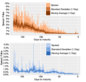Figure 3: Spread over the last six months to maturity for WTI Mini contracts (top chart) and Nikkei contracts (bottom chart)

Figure 3 clearly displays the advantage of shortterm contracts. However, as one contract per month exists for WTI, it also reveals that at least the last three contracts may have similar spreads at times. Considering long-term trading strategies, the acquisition of near contract positions create a high probability of necessary future rolls. This effect appears even stronger for different Nikkei contracts. Although there are frequently high spreads for distant futures, the high fluctuation may yield opportunities as well.

3.1         Spread composition analysis

High spreads are a symptom of market illiquidity. However, they do not automatically represent a similarly disadvantageous situations for both, buyers and sellers. For example, it is absolutely possible that a high spread of a future contract is an expression of a low supply for either long or short positions in comparison to other contracts. Still, the other side may offer attractive prices anyhow. That is the reason why an alignment of spread structures of all contracts is a reasonable step to identify trading opportunities. Therefore, a robust estimation for evolutions of the log prices is applied that generate the least absolute residuals.

Let A^F_t ^τ and B^F_t ^τ be the ask and bid log prices of F_τ at time t. The evaluation of the estimated log price X_t+1 is given by

dXt+1 RX

F∈F

Figure 4 shows the application of the robust quote estimation for the two presented WTI contracts. By interpreting all current contracts, price evolutions are computed that are placed between ask and bid prices. This creates comparable quotes for all future contracts. The differences of ask, bid and robust estimation enables the separate rating of supply and demand. For instance, the significant increase of the spread at April 24 for the December contract is primarily generated by an unfavorable ask price that cannot be traced back to a general movement. The bid price does not show any illiquidities in this case.

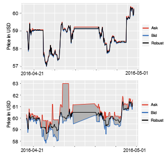Figure 4: Robust quote estimation

The resulting time series is mandatorily less volatile than both, ask and bid quotes. It only contains the minimum movement that both time series make and is robust concerning every one-sided break.

This also enables to separate non-exploitable mean reverse tendencies from real mispricings. This property will be used to evaluate under- and overvaluations in chapter 4.

3.2         Relation between spread and maturity

To formally include the remaining time span of a contract, let D ⊂ _Z be the set of durations. Let d_τ : T → _D with d_τ(t) = τ − t be the remaining time span between a time t and the maturity date τ of a future contract

F_τ.

Let dτ ∈ _D be the time interval between maturities of two consecutive future contracts. It is assumed to be constant for a future class (e.g. 1 month for WTI).

Let c: D → _R with c(d),d ≥ 0 then be the average observed trading costs that incur d time steps before the maturity.

Further, let

              c(d) = c(0)+c(dτ) +         c(d +dτ)           ∀ d < 0.      (4)

                              | {z }                   | {z }

                         Future roll cost          Liquidation cost

be the trading costs for an exceeded maturity. Future rolls consist of two trades: closing the expiring position at the last valid point before the corresponding maturity (t = c(0)) and re-opening the same position in a the consecutive contract (c(dτ)). The actual liquidation itself must be included as well and is delayed by dτ. Therefore, the overall trading cost is a sum of three values as shown in equation 4. Figure 6 illustrates these additional future roll costs for exceeded maturities.

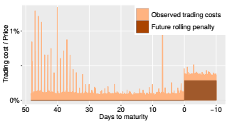Figure 5: The average trading costs c(d) over the last 50 days for WTI Mini contracts are displayed.

An exceeded maturity results in additional trades by future rolling. Therefore, the expected trading costs increase considerably for t < 0.

It can be summarized that the a low future roll probability opposes low trading costs – the least costs will generally arise in a balance between these objectives. The probability of future rolls not only depends on maturities but is primarily based on the relationship between maturity and trading frequency. Therefore, statistical information about the trading strategy must be evaluated.

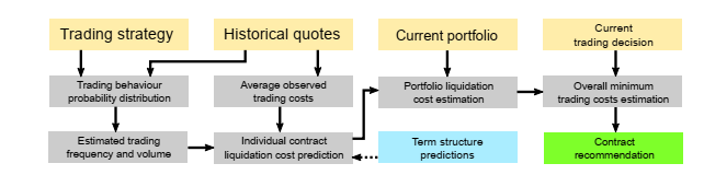Figure 6: Overview over the evaluation pipeline that leads to a contract recommendation for a given trading

decision.

3.3         Statistical trading strategy evaluation

Depending on the trading strategy, prospective trading times may be perfectly predictable. Even if there are no temporal connections, statistical methods allow the estimation based on past observations. Thus, it is assumed that a probability density function of the number of trades per time interval can be computed. In this case, it is assumed to be normally distributed with an average interval between two trades µ and a standard deviation σ. These values enable the calculation of the number of trades up to a prospective point in time. The time of the n-th upcoming trade is then represented by a random variable t_n ∼ N (t +nµ,nσ) for the last observed trading time t. The expected number of trades in an interval from s to t is ^t−_µ^s with a standard deviation of ^t−_µ^s · σ.

3.4         Portfolio liquidation costs

Next to immediate trading costs, the attractivity of contracts is strongly connected to the question how expensive the liquidation of the acquired position will be. This section focuses on the prediction of these costs. A minimization procedure is introduced with regard to the contract selection problem. It is based on the evaluation of the following information:

• future contract positions in portfolio
• estimation of spread fraction (section 3.1)
• estimation of trading cost function c (section

3.2)

• statistical information frequency and volume ofthe underlying trading strategy (section 3.3)

To connect the trading cost function c with the statistical information, we define v : T ×_T ×_T → _R to be expected trading costs. The value v(τ,t,s) displays the trading cost estimate for a future contract F_τ at time t at calcuation time s with s < t. These costs are independent from s for this first researched method and directly arise from the average observed trading costs:

                                      v(τ,t,s) = c(τ − t).                                 (5)

The future trading costs can be predicted by convoluting the probability density function f (in this case a normal-distributed approximation) and a given estimate v. The temporal uncertainty rises with increasing variance of the distribution for larger distances. This effect reduces the accuracy for more distant predictions that reveals itself by observably smoother movements representing the convolution kernel. The function C_τ : T → _R illustrates this relationship and enables the estimation of transaction costs of prospective trades at an approximate time t with the information of time s by

E(6)

∞

1

                             =         −∞ q2πt−^{s ·} σ2

_µ

                                                             

• exp− x2  · v(τ,t +x,s) dx. (7)

 2t−s · σ2  µ

In summary, statistical information about the trading strategy, observed trading costs and the estimated probability of future roll costs are weighted to calculate the most likely trading costs for a prospective trading decision.

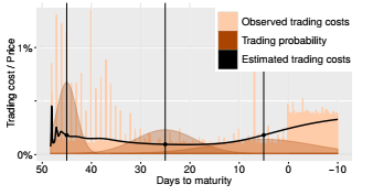Figure 7: Estimated trading costs E(C_τ (t) | F_s) for future F_τ 55 days before its maturity and ^σ_µ = ₅¹. Normal distributions for three exemplary points (45, 25 and 5 days left) are schematically figured to denote the uncertainty of the effective trading time.

The diverse trading cost effects are exemplarily demonstrated in Figure 7. It shows predictions for uprising trades for a future contract 48 days before its maturity. While the anticipated market liquidity prognosticates averagely lower costs up to 20 days before the maturity, the increased probability of future rolls yields higher estimates afterwards. While near forecasts apparently embed short-term fluctuations, estimated trading costs for distant trading events are strongly smoothed.

Indeed, these predictions are only suitable to calculate trading costs for discrete future contracts. However, individual estimates can be applied to compare different outcomes in complex scenarios of many consecutive trading decisions. This enables the evaluation of all potential executions and yields the opportunity of a trading cost minimization by prioritizing these estimates. An efficient procedure to calculate the optimal order in such a scenario is introduced in the following.

3.5         Minimizing of portfolio liquidation costs

In the following, the minimum liquidation costs by partial successive trades of a given portfolio iares measured. They are computed by an iterative calculation of optimal liquidation orders for sub-portfolios according to the dynamic programming principle. Starting with the complete portfolio, possible trading decisions are converted to orders that are used to successively remove positions. By comparing each path, an optimal trading path can be evaluated for every sub-portfolio and accordingly, for the empty portfolio. The optimal first liquidation step for the given portfolio is then revealed by the first step of the path with overall minimum trading costs.

Let the set of necessary transactions for the full liquidation of a given portfolio with N futures at time t ∈ T be given by Lt = {L1t ,L2t ,…,LNt } ∈ NN0 .

Let C_s (L_t) ∈ _R at time s ∈ _T,s ≤ t be the estimate of the trading costs for all transactions in L_t.

These transactions will happen at sequent points in future. As described, their order and their costs are predicted recursively. The remaining trading costs are for an empty portfolio have obviously the value 0:

j

C (L_t) = 0 if L_t = 0 ∀ j ∈ [1,N].        (8) _s

For every sub-portfolio, there may be up to N + 1 actions for each upcoming trading decision:

• if the direction of the order (long or short) iscontrary to an existing position of the N given futures, a position of L_t can be reduced (actions will be indexed by j = [1,N])
• choose a different transaction with minimal trading costs that does not contribute to the portfolio liqudation (indexed by j = 0)

The latter case might be reasonable if a future provides significantly better trading conditions, but it always increases the probability of future rollings as the number of necessary liquidation steps remains from t to the next trading decision at time t + µ. Therefore,

L_t+µ = L_t and accordingly

C L_t+µ = C (L_t) if j = 0. (9) _s

holds. In the other case, contracts of the future with maturity τ_j are liquidated (j = [1,N]). The gener-

           ated trading costs E C_τj (t) | F_s contribute to the overall estimation. They are added to result of the costs for the partial liquidation of the sub-portfolio.

Let the function L: Z^N × F → _Z^N represent contract liquidation. For a given portfolio in Z^N , it returns a portfolio with a reduced position in a specific future of F. The overall trading costs are defined by

C Lt+µ = Cs L Lt,τj s

                                     +E C_τj (t) | F_s            if j ∈ [1,N].            (10)

The estimated costs E C_τj (t) | F_s for the liquidation of the specific contract are added to liquidation

      costs of the residual sub-portfolio L L_t,τ_j .      These cases can be summarized to one evaluation method for the minimum liquidation costs:

 0          Cs (Lt) C Lt+µ = minj∈[0,N]∞ s     Cs L Lt,τj          +    E(Cτ(t) | Fs) 

j if Lt = 0 ∀ j ∈ [1,N] if j = 0 if Lit = 0 else. (11)

Equation 11 contains four cases, three of them are already explained. Only the third case which assigns infinite trading costs to the acquisition of positions for already liquidated contracts has not yet been mentioned. This (obviously wrong) estimate avoids the examination of further transactions after a successful liquidation. Thus, the resulting portfolio is always empty and therefore, the recursive evaluation will always stop its calculation with case one (zero transaction costs for an empty portfolio).

Every sub-portfolio can be reached by a finite number of different order combinations. The dynamic programming principle grants all possible paths to be evaluated. The resulting trading path has the minimum transaction costs according to all intermediate predictions. All in all, O(t_max · ^Q_i|^L₌₁^| Lⁱ_t) elements must be calculated. The best path can then easily be calculated by backtracking.

The selection of the best liquidation points is unambiguous for a single future when all future costs for its contract are predicted. The best liquidation is directly specified by the order subset with the minimum cumulated trading costs. The complexity arises when several liquidations seem to be optimal at the same time. The best compromise may significantly differ from a greedy selection strategy. As every future generates a new dimension in our evaluation table, such collisions become more probable when more futures are taken into consideration. The task of finding the optimal path for a single future is trivial, the complexity lies in effecting a compromise between conflicting future liquidations. The resulting path for one future is directly specified by the subset of trades with the minimal cumulated trading costs. However, possible collisions in which several transactions seem optimal at the time yield the problem of selecting specific ones. Therefore, the actual decision is based on the evaluation of all further trading steps as well. It is then given by the first trade of the best trading path.

The process of avoiding liquidations due to better trading costs of other acquisitions extends the time until the portfolio is cleared. Therefore, no finite point in time can be identified and the theoretical number of recursions has no limit. However, as future roll costs cumulate for long-running positions, liquidations of contracts near to their maturity are automatically preferred. The recursive date extension will not exceed t_max = max(s +k · µ,τ_k) with k successive futures for this reason.

4          Mean reverse inefficiencies

The following researches focus on the relationship between a spot price S_t the concerning future prices F_t,τ. We expect the future prices to converge to the spot price S_t with a simplified cost-of-carry approach. The differences are explained by specific general interest rates r_t,τ, so that

                                      Ft,τ = St · ert,τ·(τ−t).                               (12)

Several finance products are only traded as futures, so that spot prices must be approximated by the evaluation of future prices. The following approach averages interest rates between all future combinations. The spot price can be extrapolated to the current time:

lnFt,τi − lnFt,τj

                             rt,τ = avgi,j _{τi − τj}                    (13)

The interest rates between spot prices and future prices may strongly fluctuate in short periods. The set of different contract prices is referred to as term structure and several researches concerning its internal systematics have been proposed [9, 10]. As even the smallest under- or overvaluations may be used to enhance the performance of a trading strategy, an ineffiency analysis is a crucial step during the future selection process. For this purpose, it will be analysis whether cointegration between the related price series exist. Different from pure arbitrage strategies, there is no lower limit for the intensity of these inefficiencies. They do not need to be high enough to counterbalance additionally emerging trading costs as all trading decisions are already settled. However, the success of this method does not only require the existence of mean reverse effects but also their persistence to ensure a measurable predictability.

We assume the deviations from the average interest rate dr_t,τ to be potentially inefficient. In case of over- or undervaluations, mean reverse reactions should be taken into consideration. Therefore, we try to characterize the term evolutions of dr_t,τ by Ornstein-Uhlenbeck processes with

                           dr_t,τ = θ_τ µ_τ ⁻ dr_t−µ,τ dt +σ_τdW_t                              (14)

The potential mispricings dr_t,τ converge to the level µ_τ with the mean reversion speed θ_τ with a standard Wiener process (W_t)_t∈_T. σ_τ represents the influence of random noise. The parameters of this Ornstein-Uhlenbeck process are fitted with a maximum likelihood estimation [11]. The estimated approximation β_t,τ can be used to introduce a future counterbalance of mispricings to the average interest rate in the calculation of v(τ,t,x) (see Equation 6):

t,τ             t,τ
 c((τ − t) − x)+βt,τ               for a buy v(τ,t,x) =  c((τ − t) − x) − βt,τ for a sell  	(16)

                                β      = F       · edrt+µ,τ−drt,τ                                       (15)

By the modification of v(τ,t,x), the acquisition of a presumably overvalued future contract is penalized in the same way in which a sell of such a future is favored.

5          Results

The objective to reduce trading costs in futures markets by selecting specific futures is targeted by two introduced strategies. They are compared with the established front month rolling strategy for a detailed analysis. This evaluation is based on a Monte Carlo simulation with 10000 tests for each strategy that are based on sets of 100 random trading decisions each. These simulations use real time data from the time period from July 2015 to January 2016.

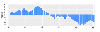Figure 8: Random portfolio series created by the first 50 trades of an exemplary simulation

Figure 8 shows the resulting portfolio after the first 50 trades of a simulation with a constant volume of one position. Accordingly, the shown portfolio evolution requires 50 contract selections at preassigned times. The result of the front month rolling strategy is shown schematically in Figure 9.

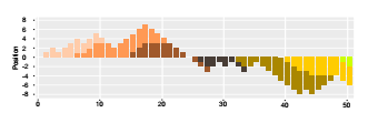Figure 9: Portfolio evolution of front month rolling strategy

Every color transition represents the change to the subsequent future. Noticeable is the periodic process in which no future is specifically preferred. As every contract is applied for one month, the number of trades is directly dependent from the trading frequency during this period. There are always not more than two different futures in the portfolio. This is induced and without exception, because overlaps directly cause future rollings in this case.

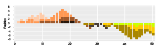Figure 10: Portfolio evolution of the minimum trading cost contract selection

Figure 10 shows the conversion of trading decisions with the introduced minimum spread approach. The preferred contract changes frequently and yield a more diverse composition with occasional formations with more than two contracts. The expected overall transaction costs are temporary estimated to be the lowest for contracts whose maturity is more than one month in the future, so that transactions partially happen noticeably earlier.

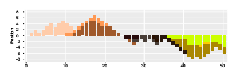Figure 11: Portfolio evolution of the minimum trading cost contract selection with the Ornstein-Uhlenbeck modification

Mean reverse predictions are added to the selection mechanism in Figure 11. The OrnsteinUhlenbeck model favors some maturities and leads to situation where some futures are almost skipped. This behavior seems likely as some futures might be seen as under- or overvalued. Even small trading costs might be no compensation in these cases.

The following research examines five different strategies:

1. Front Month rolling strategy
2. Min Spread: strategy that minimizes trading costs as described in chapter 3.5
3. Ornstein-Uhlenbeck: the minimum trading costestimation (chapter 3.5) with an additional mean reverse expectation term calculated with an Ornstein-Uhlenbeck model
4. Min Spread (SAB): Method 2, but all trading costevaluations are based on processed spread data according to the ask / bid separation introduced in chapter 3.1. The term SAB stands for a separate ask / bid quote analysis during the selection process.
5. Ornstein-Uhlenbeck (SAB): Method 3 with thesame ask / bid separation

Table 1: Performance of random sets of trading decisions on three commodities measured in index points.

        Return                 Front Month           Min Spread                     Ornstein-Uhlenbeck

WTI	2.6695	2.5692		3.1958
Natural Gas	-0.1542	0.0245		-0.0625
Silver	0.6951	1.0625		1.4265
Costs	Front Month	Min Spread		Ornstein-Uhlenbeck
WTI	1.4896	1.4126		1.5533
Natural Gas	0.5045	0.3782		0.5913
Silver	1.2405	1.0863		1.5235
Return	Min Spread (SAB)		Ornstein-Uhlenbeck (SAB)
WTI	2.9684		4.1251
Natural Gas	0.3118		0.8352
Silver	1.2014		1.6495
Costs	Min Spread (SAB)		Ornstein-Uhlenbeck (SAB)
WTI	1.3840		1.7802
Natural Gas	0.5403		0.4821
Silver	1.2114		1.2247

Table 2: Performance of random sets of trading decisions on three national index futures.

        Return                Front Month           Min Spread             Ornstein-Uhlenbeck

S&P 500	-31.8806	-28.4124		-19.1266
Nikkei 225	-760.1611	-680.2393		-580.1591
DAX	-74.1688	-61.5443		-40.5191
Costs	Front Month	Min Spread		Ornstein-Uhlenbeck
S&P 500	35.1198	30.9552		35.9812
Nikkei 225	712.1519	663.0504		634.9534
DAX	80.1419	70.4560		74.2401
Return	Min Spread (SAB)		Ornstein-Uhlenbeck (SAB)
S&P 500	-5.9915		4.1958
Nikkei 225	-531.0053		-579.5910
DAX	-10.5242		20.5994
Costs	Min Spread (SAB)		Ornstein-Uhlenbeck (SAB)
S&P 500	32.7817		35.8914
Nikkei 225	649.9088		691.1145
DAX	70.1414		75.0079

The Tables 1 and 2 show the results of Monte Carlo simulations for the different contract selection strategies. Averaged returns and trading costs are depicted for three commodities and three national indices. The cells show cumulated values that are averaged over all simulations with 100 trades each during June 2015 to January 2016.

A return of -760 points with a cost value of 712 points (Nikkei, Front Month) i.e. implies an average

loss of approximately 7 index points per trade that is mainly created by a spread near 7 index points. The loss is expected as the simulations are based on 100 random trades. The corresponding minimum spread approach reduces the cumulated trading costs to 663 points and generated an average loss of 680 points for the same 100 random trading events. The implication of mean reverse tendencies generally increases trading costs, but nevertheless accomplishes higher returns in five cases. These apparently contradicting results encourage the consideration that the term structure temporarily shows mean reverse inefficiencies.

The separation of spreads to supply and demand achieves further trading cost reductions in some cases. These are interestingly more noticeable in the minimum spread approach, the Ornstein-Uhlenbeck method hardly benefits in this category. The return raises clearly in exchange in some cases. The front month rolling strategy averages at a return of -74 points for the DAX index, but generates a win of over 20 points for the improved Ornstein-Uhlenbeck approach. Holding the same positions in different contracts results in a difference of almost 100 index points during the reviewed half year. Especially the newly introduced trading cost separation enhances the result in this case, raising it by approximately 60 points.

6          Conclusion

The selection of specific contracts is a mandatory step in futures markets that may have a huge impact on trading costs and return. Due to a complex spread structure, there are conflictive reasons to acquire contracts with near or distant maturities – the optimal selection depends on many factors. This research opposes five different selection strategies that show considerable disparities in their performance.

The study reveals that a statistical analysis of the used trading strategy and its effects on the portfolio evolution can significantly improve the performance. Therefore, not only detailed analyses of trading times and frequencies but also estimations of upcoming trading costs are contributive. Of course, this advantage requires trading events to be at least approximately predictable. The separate research on ask and bid prices for buy and sell events furtherly improve the trading performance. This holds for commodities as well as for national index futures. The introduction of mean reverse motions after possible over- or underreactions lead to higher trading costs as well as to higher return in the Monte Carlo simulation. On the one hand side, the objective of cost minimization is degraded by the introduction of further influences. On the other hand side, the consideration of over- or undervaluations increases the average return and suggests their existence in the reviewed interval.

1. V. Grossmann and M. Schimmler, “Portfolio-based contract selection in commodity futures markets,” in Computational Intelligence (SSCI), 2016 IEEE Symposium Series on. IEEE, 2016, pp. 1–7.
2. H. Geman and C. Kharoubi, “Wti crude oil futures in portfolio diversification: The time-to-maturity effect,” Journal of Banking & Finance, vol. 32, no. 12, pp. 2553–2559, 2008.
3. B. Cornell and K. R. French, “The pricing of stock index futures,” Journal of Futures Markets, vol. 3, no. 1, pp. 1–14, 1983. [Online]. Available: http://EconPapers.repec.org/RePEc:wly:jfutmk:v:3:y:1983:i:1:p:1-14
4. H. Hsu and J. Wang, “Price expectation and the pricing of stock index futures,” Review Of Quantitative Finance and Accounting, 2004.
5. E. S. Schwartz, “The stochastic behavior of commodity prices: Implications for valuation and hedging,” Journal of Finance, vol. 52, no. 3, pp. 923–73, 1997. [Online]. Available: http://EconPapers.repec.org/RePEc:bla:jfinan:v:52:y:1997:i:3:p:923-73
6. K. Tang and W. Xiong, “Index investment and the financialization of commodities,” Financial Analysts Journal, vol. 68, no. 5, pp. 54–74, 2012.
7. E. F. Fama, “Efficient Capital Markets: A Review of Theory and Empirical Work,” Journal of Finance, vol. 25, no. 2, pp. 383–417, May 1970. [Online]. Available: https://ideas.repec.org/a/bla/jfinan/v25y1970i2p383-417.html
8. G. H. Wang, J. Yau et al., “Trading volume, bid-ask spread, and price volatility in futures markets,” Journal of Futures markets, vol. 20, no. 10, pp. 943–970, 2000.
9. J. C. Cox, J. E. Ingersoll Jr, and S. A. Ross, “A theory of the term structure of interest rates,” Econometrica: Journal of the Econometric Society, pp. 385–407, 1985.
10. L. P. Hansen and R. J. Hodrick, “Forward exchange rates as optimal predictors of future spot rates: An econometric analysis,” journal of Political Economy, vol. 88, no. 5, pp. 829–853, 1980.
11. J. C. G. Franco, “Maximum likelihood estimation of mean reverting processes,” Real Options Practice, 2003.

(Click to view)

(Click to view)