1. Introduction

The purpose of the paper is to provide a comparative study of two types of adaptive consensus control schemes (Controller I and Controller II) of multi-agent systems composed of fully actuated mobile robots which are described as a class of EulerLagrange systems [22] on directed network graphs. Controller I is constructed based on the notion of inverse optimal H_∞ control criterion [23], [24], and Controller II is synthesized without H_∞ control criterion. Controller I is derived as a solutios of certain H_∞ control problem, where estimation errors of tuning parameters are considered as external disturbances to the process. Asymptotic properties, stability and robustness to unknown parameters are discussed for those two control strategies (Controller I and Controller II).
Motivated by crowd behaviors of animals, birds and fish, cooperative control problems of multi-agent systems are active research fields, and plenty of control strategies have been proposed in those areas, such as formation control, task assignment, traffic control, and scheduling et al. (for example, [1]-[11]). Among those, distributed consensus tracking of multi-agent systems with restricted communication networks, has been a basic and important issue, and various research results have been developed for various processes and under various conditions such as [1], [12][21]. In those works, adaptive control methodologies were also investigated in order to deal with uncertainties of agents, and stability of control systems was assured via Lyapunov function analysis. Furthermore, robustness properties of the control schemes were also examined. However, so much attention does not have been paid on control performance such as optimal property or transient performance in those research works, and especially, the case of multi-agent systems composed of processes with unknown and different system parameters on directed information network graphs, does not have been investigated in detail in the previous works.

The proposal of Controller I is an extension of our previous work [25], [26], in which the first-order or second-order linear or nonlinear regression models on directed network graphs were considered. This manuscript is also an extended version of the conference paper [1] (proposal of Controller I), and especially the present paper adds a comparative study of the two types of adaptive consensus control strategies (proposal and comparison of Controller I and Controller II), and highlights robustness properties of Controller I.

• Multi-Agent Systems and Network Graphs

Mathematical preliminaries on information network graph of multi-agent systems are summarized [17], [20], [21]. As a model of interaction among agents, a weighted directed graph G = (V, E) is considered,

where V = {1, ··· , N} is a node set which corresponds to a set of agents, and E ⊆ V × V is an edge set. An edge (i, j) ∈ E means that agent j can obtain information from i, but not necessarily vice versa. In the edge (i, j), i is called as a parent node and j is called as a child node, and the in-degree of the node i is the number of its parents, and the out-degree of i is the number of its children. An agent which has no parent (or with the in-degree 0), is denoted as a root. A directed path is a sequence of edges in the form (i₁,i₂), (i₂,i₃), ··· (∈ E), where i_j ∈ V. The directed graph is called strongly connected, if there is always a directed path between every pair of distinct nodes. A directed tree is a directed graph where every node has exactly one parent except for a unique root, and the root has directed paths to all other node. An directed spanning tree G_S = (V_S, E_S) of the directed graph G = (V, E) is a subgraph of G such that G_S is a directed tree and

VS = V.

Associated with the edge set E, a weighted adjacency matrix A = [a_ij] ∈ R^N×N is introduced, and the entry a_ij of it is defined by

⁽ > 0 : (j, i) ^{∈ E}, ^{aij =} 0 : otherwise.

For the adjacency matrix A = [a_ij], the Laplacian matrix L = [l_ij] ∈ R^N×N is defined such as

N

X

                             lii =              aij,

j =1 j , i

l_ij = −a_ij, (i , j).

Laplacian matrix has at least one zero eigenvalue and all nonzero eigenvalues have positive real parts. Especially, the Laplacian matrix has a simple 0 eigenvalue with the associated eigenvector 1 = [1···1]^T , and all other eigenvalues have positive real parts, if and only if the corresponding directed graph has a directed spanning tree.

In this manuscript, a consensus control problem of leader-follower type is considered, where y₀ is a leader which each agent i ∈ V should follow (i is called a follower). Concerned with the leader, a_i0 is defined such as

              ^_ > 0    :       leader⁰s information is available



a_i0 = ^_                     to follower i,                                         (1)

             ^_ 0      :     otherwise,

and from a_i0 and L, the matrix M ∈ R^N×N is defined by

                         M = L+diag(a₁₀··· a_N0).                                    (2)

It is shown that −M is a Hurwitz matrix, if and only if 1. at least one a_i0 (1 ≤ i ≤ N) is positive, and 2. the graph G has a directed spanning tree with the root i = 0.

Hereafter, we assume that

1. The graph has a directed spanning tree with theroot i = 0.
2. At least one a_i0 (1 ≤ i ≤ N) is positive, that is, the information of the leader y₀ (y˙₀, y¨₀), is available to at least one follower i.
3. For the leader, y₀, y˙₀, y¨₀ are uniformly bounded.

In the following, two adjacency matrices A = [a_ij],

C = [c_ij] ∈ R^N×N are introduced for a directed graph G, and the corresponding matrices are denoted as L_a, L_c (Laplacian matrices), and M_a, M_c, respectively.

3 Problem Statement

A multi-agent system composed of N fully actuated mobile robots which are described as a class of EulerLagrange systems [9], [10], are considered such that

M_i(y_i)y¨_i +C_i(y_i,y˙_i)y˙_i = τ_i, (i = 1, ··· , N), (3) where y_i ∈ Rⁿ is an output (a generalized coordinate), τ_i ∈ Rⁿ is a control input (a force vector), M_i(y_i) ∈ R^n×n is an inertia matrix, and C_i(y_i,y˙_i) ∈ R^n×n is a matrix of Coriolis and centripetal forces. Each component has the next properties as a Euler-Lagrange system. Properties of Euler-Lagrange Systems [22]

1. M_i(y_i) is a bounded, positive definite, and symmetric matrix.
2. M˙ _i(y_i)−2C_i(y_i,y˙_i) is a skew symmetric matrix.
3. The left-hand side of (3) can be written into

                        M_i(y_i)a_i +C(y_i,y˙_i)b_i = Y_i(y,y˙_i,a_i,b_i)θ_i,                (4)

where Y_i(y_i,y˙_i,a_i,b_i) is a known function of y_i, y˙_i, a_i, b_i (a regressor matrix), and θ_i is an unknown system parameter vector.

The control objective is to achieve consensus tracking of the leader-follower type for the unknown multiagent system (unknown θ_i) such as

yi → yj, (i, j = 1,··· , N),	(5)
yi → y0, (i = 1,··· , N),	(6)

under the limited communication structure G among agents.

4 Control Law and Error Equation

Remark 1 More generalized Euler-Lagrange systems including damping terms and gravitational forces, can be also considered in the present framework. However, for simplicity of notations, the description (3) is to be adopted hereafter, since the generalized Euler-Lagrange systems are written in the similar form to (4).

As the first step of the design of Controller I and Controller II, an estimator of y˙₀ (the leader’s information) is developed via available data from the follower i. A similar estimation procedure was presented in [16].

N

zˆ˙i(t) = −β X cij{zˆi(t)−zˆj(t)}

j =1 j , i

                                    −βc_i0{zˆ_i(t)−y˙₀(t)}+n_i0y¨₀(t),                (7)

where zˆ_i is a current estimate of y˙₀, and is synthesized from the data available to the follower i. c_ij (1 ≤ i ≤ N, 0 ≤ j ≤ N) is defined as the entry of the adjacency matrix C and (1) deduced from the directed graph G, and β > 0 is a design parameter. Associated with c_i0, n_i0 is defined such as

                    ni0 = ( 01     :: cotherwisei0 > 0,                               .       (8)

By employing the estimate zˆ_i, the control scheme is constructed as follows:

XN

y˙ri(t) = zˆi(t)−α                   aij{yi(t)−yj(t)}, j =0 j , i	(9)
si(t) = y˙i(t)−y˙ri(t),	(10)
τi(t) = Yi(t)θˆi(t)+vi(t),	(11)
Yi(t) ≡ Yi(y,y˙i,y¨ri,y˙ri),	(12)

where a_ij (1 ≤ i ≤ N, 0 ≤ j ≤ N) is defined similarly from the entry of the adjacency matrix A and (1) deduced from G, and α > 0 is a design parameter. θˆ_i is denoted as a current estimate of unknown θ_i, and v_i is a stabilizing signal which is to be determined later based on the notion of inverse optimal H_∞ control criterion (Controller I), or without H_∞ control criterion (Controller II). An estimation error between the leader y˙₀ and the estimate zˆ_i is defined by

                            z˜_i(t) ≡ zˆ_i(t)−y˙₀(t),                                     (13)

and the following relations are deduced for s_i and z˜_i.

N

z˜˙i(t) = −β X cij{z˜i(t)−z˜j(t)}

j =1 j , i

−βci0z˜i(t)+(ni0 −1)y¨0(t), Mi(yi)s˙i(t)+Ci(yi,y˙i)si(t)	(14)
= vi(t)+Yi(t){θˆi(t)−θi}.	(15)

Then, the overall representations of the multi-agent system are given as follows:

              z˜˙(t) = −β(M_c ⊗I)z˜(t)+{(N₀ −1)⊗I}y¨₀(t),           (16)

Ms˙(t)+Cs(t) = Y(t){θˆ −θ(t)}+v(t), (17) where

z˜  , z˜_N^T ]^T,      (18) s ^T,           (19)

M = block diag(M1,··· , MN ), (Mi ≡ Mi(yi)),	(20)
C = block diag(C1,··· , CN ), (Ci ≡ Ci(yi,y˙i)),	(21)
Y = block diag(Y1,··· , YN ),	(22)

         , θ_N^T ]^T,                                                         (23)

N0 = [n10,··· , nN0]T,	(24)
1 = [1,··· , 1]T,	(25)

v  , v_N^T ]^T,          (26) and ⊗ denotes Kronecker product.

5 Adaptive H_∞ Consensus Control for Euler-Lagrange Systems (Controller I)

In this section a design scheme of adaptive consensus control based on inverse optimal H_∞ criterion (Controller I) is provided. Stability analysis of the overall control system and deduction of Controller I are composed of four steps. As the first step, for stability analysis of s and the related terms, a positive function W₀ is defined such as

                                   W₀(t) = s(t)^TMs(t).                            (27)

Then, the time derivative of W₀ along its trajectory is derived as follows:

                       W˙ ₀(t) = s(t)^T[Y(t){θˆ −θ(t)}+v(t)].                (28)

By considering the evaluation of W˙ ₀ (28), the next virtual system is introduced.

s˙ = f +g1d +g2v,	(29)
f = 0,	(30)
g1 = Y, g2 = I,	(31)
d = (θˆ −θ).	(32)

The virtual system is to be stabilized via a control input v based on H_∞ criterion, where d is considered as an external disturbance to the process. For that purpose, the following Hamilton-Jacobi-Isaacs (HJI) equation and its solution V₀ are introduced.

      f 41 ^kL_gγ1V0k2 −(Lg2V0)R−1(Lg2V0)T^+q = 0,

L V0 +                       2

(33)

1 T

V₀ =      s s,                                                                            (34)

2 where q and R are a positive function and a positive definite matrix respectively, and those are deduced from HJI equation based on the notion of inverse optimality for the given solution V₀ and a positive constant γ. The substitution of the solution V₀ (34) into HJI equation (33) yields

                                  1 T(YYT −R−1)s +q = 0.                           (35)

                           4s         γ2

From (35), R and q are obtained such as

                                               YYT                !⁻1

                                   R =          γ₂ +K          ,                           (36)

1 T

                                   q =          s Ks,                                       (37)

4

where K is a diagonal positive definite matrix (a design parameter), From R, v is derived as a solution of the corresponding H_∞ control problem as follows

(Controller I):

v = −R−1(Lg2V0)T = −R−1s

• YYT !

                            = −    +K s.                                    (38)

• γ₂

Then, via HJI equation, the time derivative of W₀ (28) is evaluated as follows:

W˙ 0 = −q −vTRv

                                           1              T

                                 + v +   R−1s         R v + 1R−1s

                                            2                           2

2kdk2 −γ2      d − 2γT2s      2,             (39) Y +γ

and it follows that s is bounded for bounded θˆ and for the stabilizing signal v (38).

Next, for stablity analysis of the estimation error z˜, a positive function V₁ is introduced such as

                     V₁ = z˜^T(P_c ⊗I)z,˜                                              (40)

                         P_cM_c +M_c^TP_c = I, (P_c = P_c^T > 0).                      (41)

There exists a positive definite and symmetric matrix P_c satisfying (41), since −M_c is Hurwitz. Then, the time derivative of V₁ along its trajectory is evaluated as follows:

V˙₁ = −βkz˜k² −2z˜^T(P_c ⊗I){(N₀ −1)⊗I}y¨₀

and it is shown that z˜ is bounded for bounded y¨₀.

Thirdly, for stability analysis of the control error y_i −y₀ and the related terms, y˜_i, y˜ are defined by

y˜i = yi −y0,	(43)
y˜ = [y˜1T, ··· , y˜NT ]T.	(44)

Then, the following relation holds

                              y˜˙ = s +z˜−α(M_a ⊗I)y,˜                          (45)

and −M_a is shown to be Hurwitz because of the assumption of the network graph G. From that property, a positive function V₂ is defined by

                     V₂ = y˜^T(P_a ⊗I)y,˜                                              (46)

                         P_aM_a +M_a^TP_a = I, (P_a = P_a^T > 0).                     (47)

Similarly to the previous case (M_c), there exists a positive definite and symmetric matrix P_a satisfying (47), since −M_a is Hurwitz. Then, the time derivative of V₂ along its trajectory is evaluated as follows:

V˙

From the three stages of stability analysis (the evaluations of W˙ ₀, V˙₁, V˙₂), the next theorem is obtained.

Theorem 1 The nonlinear control system composed of the control laws (7), (9), (10), (11), (12), (38) (Controller I) is uniformly bounded for an arbitrary bounded design parameter θˆ_i, and bounded y₀, y˙₀, y¨₀, and v is an optimal control input which minimizes the following cost functional J.

“Z t

              J(t) ≡         sup                 {q +v^TRv}dτ +W₀(t)

                           di,d2,d3∈L2          0

                                    Z t                      #

−γ2              kdk2dτ . 0 Also the next inequality holds. Z t {q +vTRv}dτ +W0(t) 0	(49)
Z t	(50)
≤ γ2                kdk2dτ +W0(0).

0

Theorem 1 denotes the properties of the proposed nonlinear control system (7), (9), (10), (11), (12), (38) (Controller I), where the tunings of θˆ is not included (or not necessarily required).

Next, the tuning law of θˆ is determined as follows: θˆ^˙(t) = Prⁿ−ΓY(t)^Ts(t)^o,          (51)

where Pr(·) is a projection operation in which the tuning parameter θˆ is constrained to a bounded region deduced from upper-bounds of kθk [27]. As the fourth step of stability analysis of the overall control system, a positive function W₁ is defined by

W₁(t) = s(t)Ts(t)+ nθˆ(t)−θoTΓ −1nθˆ(t)−θo, (52)

and the time derivative of W₁ along its trajectory is evaluated such as

                           W˙ .                    (53)

From the four stages of stability analysis (the evaluations of W˙ ₀, W˙ ₁, V˙₁, V˙₂), the next theorem is obtained.

Theorem 2 The adaptive control system composed of the control laws (7), (9), (10), (11), (12), (38), and the tuning law of θˆ (51) (Controller I), is uniformly bounded for bounded y₀, y˙₀, y¨₀, and it follows that

lim s(t) = 0.           (54) t→∞

Especially, if y¨₀(t) = 0 or the information of the leader y¨₀ is available for all followers ({(N₀ −1)⊗I}y˙₀ = 0), then it follows that

                        lim y˜(t) = lim y˜˙(t) = 0,                                (55)

                       t→∞                    t→∞

and the asymptotic consensus tracking is achieved. Otherwise, when y¨₀(t) , 0 and the information of y¨₀ is not available for all followers ({(N₀ − 1) ⊗ I}y¨₀ , 0), then the next relation holds.

ky˜k ∼ const.k, (56) ky˜˙k ∼ const.. (57)

Theorem 2 denotes the properties of the proposed adaptive control system (7), (9), (10), (11), (12), (38), (51) (Controller I), and states that the asymptotic consensus tracking is achieved under the specified condition ({(N₀ − 1) ⊗ I}y˙₀ = 0), and also shows that the approximate consensus tracking with the ratios of 1/(αβ), 1/β(> 0) is still assured, even if that condition is not satisfied ({(N₀ −1)⊗I}y¨₀ , 0).

Remark 2 It should be noted the proposed control scheme and the adaptation scheme (Controller I) are all implemented in a distributed fashion, where availabilities of signals for each agent i are highly restricted and prescribed by the directed graph G.

Remark 3 The objective of the design of Controller I, is to obtain an adaptive control structure whose stability is not seriously affected by the adaptation scheme, or whose performance is not significantly degraded by the estimation errors of the tuning parameters. For that purpose, in order to attenuate the effects of the estimation errors, the control scheme is to be deduced as a solution of certain H_∞ control problem, where L₂ gains from the estimation errors of tuning parameters to the generalized output is prescribed by a positive constant γ (design parameter).

Remark 4 Of course, J in Theorem 1 is a fictitious cost functional, since d is not an actual disturbance but an estimation error of the tuning parameter, and since it is not generally included in L²[0,∞). Nevertheless, v, which is derived as a solution for that fictitious H_∞ control problem (Controller I), attain the inequality in Theorem 1, stabilize the total system, and it means that the L² gain from the disturbance

d to the generalized output ^pq +v^T Rv is prescribed by the positive constant γ.

6 Adaptive Consensus Control for Euler-Lagrange Systems without H_∞ Criterion (Controller II)

The adaptive consensus control strategy without H_∞ control criterion (Controller II) is easily deduced by setting γ → ∞ in the synthesis of v (38) such that

                                           v = −Ks.                                       (58)

In this case, the tuning scheme of θˆ (51) is required to assure uniform boundedness of the total control system. The time derivative of W₁ (52) with the tuning law (51) gives

                             W˙ .                      (59)

Then, by applying the same stability analysis via the evaluations of W˙ ₁, V˙₁, V˙₂, the following theorem is obtained.

Theorem 3 The adaptive control system composed of the control laws (7), (9), (10), (11), (12), (58), and the tuning law of θˆ (51) (Controller II), is uniformly bounded for bounded y₀, y˙₀, y¨₀, and it follows that

lim s(t) = 0.           (60) t→∞

Especially, if y¨₀(t) = 0 or the information of the leader y¨₀ is available for all followers ({(N₀ −1)⊗I}y˙₀ = 0), then it follows that

lim y˜(t) = lim y˜˙(t) = 0, (61) t→∞ t→∞

and the asymptotic consensus tracking is achieved. Otherwise, when y¨₀(t) , 0 and the information of y¨₀ is not available for all followers ({(N₀ − 1) ⊗ I}y¨₀ , 0), then the next relation holds.

ky˜k ∼ const.k, (62) ky˜˙k ∼ const.. (63)

Remark 5 Asymptotic properties of the adaptive consensus control without H_∞ criterion ((60), (61), (62), (63) (Controller II)) are the same as the adaptive H_∞ consensus control version ((54), (55), (56), (57) (Controller I)). However, it should be noted that uniform boundedness of the overall control system via Controller II is not assured for arbitrary bounded design parameters θˆ. Instead, the tuning of θˆ (51) is necessary to attain the stability of consensus tracking by Controller II. Furthermore, Controller II in Theorem 3 does not contain an optimal property for the cost functional (49), and the inequality (50) does not hold.

7 Numerical Example

In order to show the effectiveness of the two types of adaptive consensus control schemes, numerical experiments for Euler-Lagrange systems are performed. A multi-agent system composed of simple EulerLagrange systems is considered as follows: m_iy¨_i(t) = τ_i(t), (i = 1, 2, 3),

(y₁(0) = 1, y₂(0) = 0, y₃(0) = −1),

where y_i ∈ R, τ_i ∈ R, and m_i ∈ R is an unknown system parameter. Associated with the information network structure (Fig.1), the adjacency matrix A = [a_ij](= C) and a_i0(= c_i0) are chosen such that

                                 0     1     0 

                                                   

                     A =  1  0 1 ,

                                0    1   0 

a10 = 1, a20 = a30 = 0.

The control objective is to achieve consensus tracking

yi → yj, y˙i → y˙j, yi → y0, y˙i → y˙0,

(i, j = 1, 2, 3), where the virtual leader y₀ is determined such as y¨₀ +2y˙₀(t)+y₀(t) = sint.

The design parameters are chosen as follows:

Γ = 10I, K = 5I, α = β = 10, γ_i = 1.

As system parameters m_i (i = 1 ∼ 3), we consider both time-invariant and time-varying cases such that

m₁ = 1, m₂ = 2, m₃ = 3, (time−invariant case), m₁ = f_m(t), m₂ = 2f_m(t), m₃ = 3f_m(t),

where	(time−varying case),
( 2 fm(t) =          1	0 ≤ t < 2.5, 5 ≤ t < 7.5, ··· , 2.5 < t ≤ 5, 7.5 < t ≤ 10, ··· .

Numerical simulations were carried out by utilizing MATLAB and Simulink of the MathWorks, Inc., and the solver is Dormand-Prince method with the adaptive step-size integration algorithm (ode45).

The simulation results of Controller I (Theorem

2) are shown in Fig.2 (time-invariant case) and Fig.4 (time-varying case). For comparison, the cases of Controller II (the adaptive control systems which do not contain H_∞ control scheme), are shown for both cases; Fig.3 (time-invariant case) and Fig.5 (time-varying case). In those figures (Fig.2 ∼ Fig.5), the plots were response curves of y₁, y₂, y₃ and y₀ (vertical axises) versus time t (horizontal- axises).

From those results, it is seen that Controller I (H_∞ adaptive control strategy) achieves better tracking convergence property together with robustness to abrupt changes of the system parameters compared with the non-H_∞ control scheme (Controller II), and those are owing to disturbance attenuation properties of Controller I, since the performance of Controller I is not significantly degraded by the estimation errors of the tuning parameters in the settings of both timeinvariant and time-varying cases (see also Remark 3).

8 Concluding Remarks

The comparative study of two types of adaptive consensus control (Controller I and Controller II) of multi-agent systems composed of fully actuated mobile robots which are described as a class of EulerLagrange systems on directed network has been given in this paper. Controller I is deduced based on the notion of inverse optimal H_∞ control criterion, and is derived as a solution of certain H_∞ control problem, where estimation errors of tuning parameters are considered as external disturbances to the process. On the contrary, Controller II is synthesized without H_∞ control criterion. Asymptotic properties, stability and robustness to unknown parameters are discussed for those two control strategies (Controller I and Controller II). Although asymptotic properties of those two controllers are similar to each others, Controller I achieves better tracking convergence property together with robustness to abrupt changes of the system parameters compared with Controller II, and those are owing to disturbance attenuation properties of Controller I and the problem setting of H_∞ criterion.

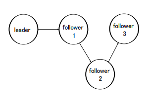Fig. 1 Information Network Graph

Time

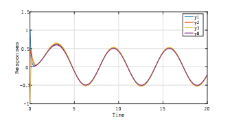Fig. 2 Simulation Result for Time-Invariant Case with

H_∞ Control Scheme (Controller I)

Time

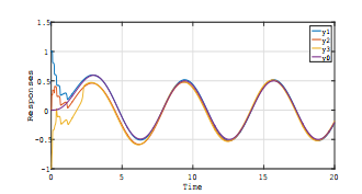Fig. 3 Simulation Result for Time-Invariant Case without H_∞ Control Scheme (Controller II)

Time

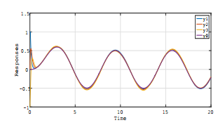Fig.4 Simulation Result for Time-Varying Case with

H_∞ Control Scheme (Controller I)

Time

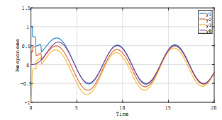Fig. 5 Simulation Result for Time-Varying Case without H_∞ Control Scheme (Controller II)

1. Y. Miyasato, ”Adaptive H1 Consensus Control of Euler-Lagrange Systems on Directed Network Graph”, Proceedings of IEEE Symposium Series on Computational Intelligence (IEEE SSCI 2016), 2016. https://doi.org/10.1109/SSCI.2016.7849871
2. M.A. Tan and K. Lewis, ”Virtual Structures for High-Precision Cooperative Mobile Robot Control”, Proceedings of the 1996 IEEE/RSJ INternational Conference Intelligent Robots and Systems, Vol.1, pp.132-139, 1996.
3. T. Balch and R.C. Arkin, ”Behavior-Based Formation Control for Multirobot Teams”, IEEE Transactions on Robotics and Automation, Vol.14, pp.926-939, 1998.
4. G. Inalhan, D.M. Stipanovic, and C. Tomlin, ”Decentralized Optimization with Application to Multiple Aircraft Coordinate,” Proceedings of the 41st IEEE Conference on Decision and Control, pp.1147-1155, 2002.
5. J. Yao, R. Ordo´nez and V. Gazi, ”Swarm Tracking Using Artificial Potentials and Sliding Mode Control”, Proceedings of the 45th IEEE Conference on Decision and Control, pp.4670-4675, 2006.
6. J. Shao, G. Xie and L. Wang, ”Leader Following Formation Control of Multiple Mobile Vehicles”, IET Control Theory Appl., Vol.1, pp.545-552, 2007.
7. R.M. Murray, ”Recent Research in Cooperative Control of Multivehicle Systems,” Journal of Dynamic Systems, Measurement, and Control, Vol.129, No.5, pp.571-583, 2007.
8. K.L. Moore and D. Lucarelli, ”Decentralized Adaptive Scheduling Using Consensus Variables, ” International Journal of Robust and Nonlinear Control,Vol.17, pp.921-940, 2007.
9. A.R. Pereira and L. Hsu, ”Adaptive Formation Control Using Artificial Potentials for Euler-Lagrange Agents”, Proceedings of the 17th IFAC World Congress, pp.10788-10793, 2008.
10. C.C. Cheah, S.P. Hou and J.J.E. Slotine, ”Region-Based Shape Control for a Swarm of Robots”, Automatica, Vol.45, pp.2406-2411, 2009.
11. Y. Miyasato, ”Adaptive H_∞ Formation Control for Euler-Lagrange Systems, Proceedings of the 49th IEEE Conference on Decision and Control, pp.2614-2619, 2010.
12. D. Kingston, W. Ren, and R. Beard, ”Consensus algorithms are input-to-state stable,” Proceedings of 2005 American Control Conference, pages 1686-1690, 2005.
13. R. Olfati-Saber, J. A. Fax, and R. M. Murray. Consensus and Cooperation in Networked Multi-Agent Systems. Proceedings of the IEEE, Vol.95, pp. 215-233, 2007.
14. W. Ren, K.L. Moore, and Y. Chen, ”High-Order and Model Reference Consensus Algorithms in Cooperative Control of Multi-Vehicle Systems,” Transaction of American Society of Mechanical Engineers, Vol.129, pp.678-688, 2007.
15. Y. Cao and W. Ren, ”Distributed Coordinate Tracking via a Variable Structure Approach – Part I : Consensus Tracking,” Proceedings of 2010 American Control Conference, pp.4744-4749, 2011.
16. J. Mei and W. Ren, ”Distributed Coordinate Tracking with a Dynamic Leader for Multiple Euler-Lagrange Systems,” IEEE Transactions on Robotics and Automation, Vol.56, pp.1415-1421, 2011.
17. W. Ren and Y. Cao, Distributed Coordination of Multi-Agent Networks, Springer, 2011.
18. G. Wen, Z. Duan, W. Yu and G. Chen, ”Consensus in Multi-Agent Systems with Communication Constraints”, International Journal of Robust and Nonlinear Control, Vol.22, pp.170-182, 2012.
19. W. Yu, W. Ren, W.X. Zheng, G. Chen and J. Lu, ”Distributed ¨ Control Gains Design for Consensus in Multi-Agent Systems with Second-Order Nonlinear Dynamics”, Automatica, Vol.49, pp.2107-2115, 2013.
20. J. Mei, W. Ren and J. Chen, ”Consensus of Second-Order Heterogeneous Multi-Agent Systems under a Directed Graph,” Proceedings of 2014 American Control Conference, pp.802-807, 2014.
21. J. Mei, W. Ren, J. Chen B.D.O. Anderson, ”Consensus of Linear Multi-Agent Systems with Fully Distributed Control Gains under a General Directed Graph”, Proceedings of the 53rd IEEE Conference on Decision and Control, pp.2993-2998, 2014.
22. M.W. Spong and M. Vidyasagar, Robot Dynamics and Control, John Wiley & Sons, 1989.
23. M. Krstic and H. Deng, ´ Stabilization of Nonlinear Uncertain Systems, Springer, 1998.
24. Y. Miyasato, ”Adaptive Nonlinear H1 Control for Processes with Bounded Variations of Parameters – General Relative Degree Case -”, Proceedings of the 39th IEEE Conference on Decision and Control, pp.1453-1458, 2000.
25. Y. Miyasato, ”Adaptive H1 Consensus Control of Multi-Agent Systems on Directed Graph”, Proceedings of the 39th IEEE Conference on Decision and Control, pp.1453-1458, 2015.
26. Y. Miyasato, ”Adaptive H_∞ Consensus Control of Multi-Agent Systems on Directed Graph by Utilizing Neural Network Approximators”, Proceedings of IFAC Workshops, ALCOSP and PSYCO 2016, 2016.
27. P.A. Ioannou and J. Sun, Robust Adaptive Control, PTR Prentice-Hall, NJ; 1996.

(Click to view)

(Click to view)