1. Introduction

In the earlier paper [1], transformer condition is used to estimate its end of life using instant data. In this paper, transformer condition is calculated using maintenance data from Indonesia Electric Company (PLN) and is interpreted using Cognitive-Artificial method. Each factor influencing the same component is assumed to have the same weight in the condition calculation. The condition is then interpreted to provide early warning system for the potential failure and to estimate the transformer end of life.

There are no single conventional method of transformer diagnosis can be used to define transformer condition accurately. Usually there are several methods combined to perform such a task. These methods are very expert-dependant and are not formulated. Therefore, an automated method for transformer condition monitoring is proposed. Using Cognitive-Artificial-Intelligence (CAI) method, the transformer condition interpretation can be accurately performed, and the expert-dependency can be reduced as well.

2.       Transformer Condition Component

Transformer condition can be calculated using some factors. These factors are shown in Figure 1 [2].

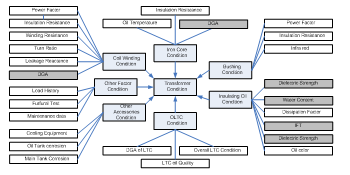Figure 1 Transformer Condition Factors [2]

Data are collected from PLN and fused to obtain part conditions, part conditions are then fused to obtain transformer condition. Figure 2 explains how transformers degrade over time.

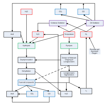Figure 2 Transformer Degradation Diagram [3]

There are two main processes of the transformer degradation process, hydrolysis and pyrolysis. Hydrolysis is related to water, while pyrolysis is related to fire. The main cause of hydrolysis is water, acids and temperature causes hydrolysis as well. Pyrolysis is caused by temperature [3].

Hydrolysis causes depolymerization of transformer insulating system, and later produces furanoid compounds, which produces carbon dioxide and carbon monoxide, which is the main cause of acids [3]. Acid will then cause hydrolysis.

Pyrolysis causes levoglucosane fragmentation, which produces diatomic oxygen. Oxygen is the cause of oxidation in cellulose and oil, which leads to hydrolysis [3]. These two degradation processes and the compounds they produce makes the transformer degradation processes accelerate over time. The impact of diatomic oxygen will be discussed in Load Tap Changer.

3.       The Mathematical Model of Arwin-Adang-Aciek-Sembiring (A3S) [4]

How knowledge grows in the system can be described using Figure 2 [4, 5]. There are two main parts of Knowledge-Growing System. The upper part of Figure 3 contains Information Fusion, while the lower part of the diagram contains knowledge fusion.

The system receives multi-source information from sensors and performs information fusion. When the information exceeds certain level of desirable Degree of Certainty, the information will be considered as knowledge.

The knowledge will be fused with the existing knowledge in the knowledge part of the system to obtain new knowledge and is stored. When the new knowledge exceeds certain level of DoC, it will become the ultimate knowledge.

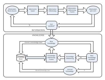Figure 3 Knowledge-Growing System [5]

A3S (Arwin-Adang-Aciek-Sembiring) algorithm [5] is information fusion algorithm based on Bayesian Inference Method. When a problem occurs, the system collects information and fuses them to produce new knowledge. A3S starts with (1).

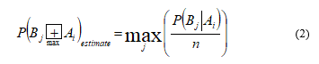
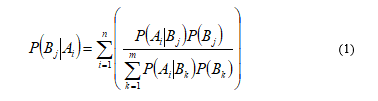Where  is the probability of is true given the presence of the fusion or combination of all events [4]. Maximum A Posteriori (MAP) is determined by (2)

It is then simplified to become (3)

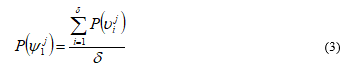Where  will be the New Knowledge Probability Distribution (NKPD) at a certain observation time γ₁ [4]. The new knowledge will be obtained by applying (4).

The system will keep collecting information (NKPD) on each observation, , …, , …,  [4]. The inferencing can be determined using (5).

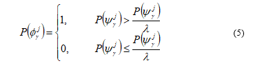Where  is inferencing of each information to the knowledge distribution.

Information-inferencing fusion will be calculated using OMA3S method, a dynamic version of A3S resulting NKPD over Time (NKPDT) [4].

4.       Transformer condition calculation

System’s block diagram is shown in Figure 4.

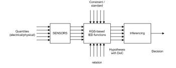Figure 4 System’s block diagram

Data is collected using sensors and is compared to standards and relation.  The system fills the observation table using (1). After each observation, there will be new knowledge shown by New Knowledge Probability Distribution (NKPD). Each NKPD is fused with the previous NKPD to produce NKPD over time (NKPDT). Decisions are made based on NKPDT.

There are two kinds of faults in transformers. They are electrical faults and thermal faults [9]. Electrical faults are Partial Discharge, Low-Energy Discharge, and High Energy Discharge, while thermal faults are Thermal-Low and Thermal-High [9]. The proposed method is tested using previously published DGA dataset, which is classified based on the identified fault [9]. Table 1 shows Partial Discharge dataset, Table 2 shows Low-Energy Discharge, Table 3 shows High-Energy Discharge, Table 4 shows Thermal-Low, and Table 5 shows High-Energy Discharge.

Table 1 Partial Discharge dataset [9].

No.	H2	CH4	C2H6	C2H4	C2H2	CO
1	32930	2397	157	0	0	313
2	37800	1740	249	8	8	56
3	92600	10200	0	0	0	6400
4	8266	1061	22	0	0	107
5	9340	995	60	6	7	60
6	36036	4704	554	5	10	6
7	33046	619	58	2	0	51
8	40280	1069	1060	1	1	1
9	26788	18342	2111	27	0	704

Table 2 Low-Energy Discharge dataset [9].

No.	H2	CH4	C2H6	C2H4	C2H2	CO
1	78	20	11	13	28	0
2	305	100	33	161	541	440
3	35	6	3	26	482	200
4	543	120	41	411	1880	76
5	1230	163	27	233	692	130
6	645	86	13	110	317	74
7	60	10	4	4	4	780
8	95	10	0	11	39	122
9	6870	1028	79	900	5500	29

Table 3 High-Energy Discharge dataset [9].

No.	H2	CH4	C2H6	C2H4	C2H2	CO
1	440	89	19	304	757	299
2	210	43	12	102	187	167
3	2850	1115	138	1987	3675	2330
4	7020	1850	0	2960	4410	2140
5	545	130	16	153	239	660
6	7150	1440	97	1210	1760	608
7	620	325	38	181	244	1480
8	120	31	0	66	94	48
9	755	229	32	404	460	845

Table 4 Thermal-Low dataset [9].

No.	H2	CH4	C2H6	C2H4	C2H2	CO
1	1270	3450	520	1390	8	483
2	3420	7870	1500	6990	33	573
3	360	610	259	260	9	12000
4	1	27	49	4	1	53
5	3675	6392	2500	7691	5	101
6	48	610	29	10	0	1900
7	12	18	4	4	0	559
8	66	60	2	7	0	76
9	1450	940	211	322	61	2420

 Table 5 Thermal-High dataset [9].

No.	H2	CH4	C2H6	C2H4	C2H2	CO
1	8800	64064	72128	95650	0	290
2	6709	10500	1400	17700	750	290
3	1100	1600	221	2010	26	0
4	290	966	299	1810	57	72
5	2500	10500	4790	13500	6	530
6	1860	4980	0	10700	1600	158
7	860	1670	30	2050	40	10
8	150	22	9	60	11	0
9	400	940	210	820	24	390

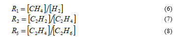
In order to analyze the DGA, there are several ratios required, they are [5]:

These ratios are put into groups based on Table 6.

Table 6 Gas Ratio grouping [9].

	R2	R1	R5
< 0.1	0	1	0
0.1 – 1.0	1	0	0
1.0 – 3.0	1	2	1
> 3	2	2	2

Estimated faults can be determined using the rules shown in Table 7 [9].

Table 7 Gas Ratio grouping [9].

No.	Characteristic Fault	R2	R1	R5
0	No fault	0	0	0
1	Partial Discharge	0 or 1	1	0
2	Low-Energy Discharge	1 or 2	0	1 or 2
3	High-Energy Discharge	1	0	2
4	Thermal-Low	0	0 or 2	0 or 1
5	Thermal-High	0	2	2

Datasets are made into Ratios and are put into groups as shown in Table 8 to Table 12.

Table 8 Ratios: Partial Discharge.

Ratio			Ratio Group
R1	R2	R5	R1	R2	R5
2.72	0.01	2.67	1	2	0
2.30	0.00	4.66	1	1	0
1.69	0.03	1.00	0	2	2
27.00	0.25	0.08	0	2	0
1.74	0.00	3.08	0	1	0
12.71	0.00	0.34	0	1	0
1.50	0.00	1.00	1	0	0
0.91	0.00	3.50	1	1	0
0.65	0.19	1.53	0	0	0

Table 9 Ratios: Low-Energy Discharge.

Ratio			Ratio Group
R1	R2	R5	R1	R2	R5
0.26	2.15	1.18	0	1	1
0.33	3.36	4.88	0	2	2
0.17	18.54	8.67	0	2	2
0.22	4.57	10.02	0	2	2
0.13	2.97	8.63	0	1	2
0.13	2.88	8.46	0	1	2
0.17	1.00	1.00	0	1	1
0.11	3.55	inf	0	2	2
0.15	6.11	11.39	0	2	2

Table 10 Ratios: High-Energy Discharge.

Ratio			Ratio Group
R1	R2	R5	R1	R2	R5
0.20	2.49	16.00	0	1	2
0.20	1.83	8.50	0	1	2
0.39	1.85	14.40	0	1	2
0.26	1.49	inf	0	1	2
0.24	1.56	9.56	0	1	2
0.20	1.45	12.47	0	1	2
0.52	1.35	4.76	0	1	2
0.26	1.42	inf	0	1	2
0.30	1.14	12.63	0	1	2

Table 11 Ratios: Thermal-Low.

Ratio			Ratio Group
R1	R2	R5	R1	R2	R5
2.72	0.01	2.67	2	0	1
2.30	0.00	4.66	2	0	2
1.69	0.03	1.00	2	0	1
27.00	0.25	0.08	2	1	0
1.74	0.00	3.08	2	0	2
12.71	0.00	0.34	2	0	0
1.50	0.00	1.00	2	0	1
0.91	0.00	3.50	0	0	2
0.65	0.19	1.53	0	1	1

Table 12 Ratios: Thermal-High.

Ratio			Ratio Group
R1	R2	R5	R1	R2	R5
7.28	0.00	1.33	2	0	1
1.57	0.04	12.64	2	0	2
1.45	0.01	9.10	2	0	2
3.33	0.03	6.05	2	0	2
4.20	0.00	2.82	2	0	1
2.68	0.15	inf	2	1	2
1.94	0.02	68.33	2	0	2
0.15	0.18	6.67	0	1	2
2.35	0.03	3.90	2	0	2

Ratio Groups are arranged into observation table as shown in Table 13 to Table 17 where:

• H_PD: Hypothesis Partial Discharge.
• H_LE: Hypothesis Low-Energy Discharge.
• H_HE: Hypothesis High-Energy Discharge.
• H_TL: Hypothesis Thermal-Low.
• H_TH: Hypothesis Thermal-High.

Table 13 Observation: Partial Discharge.

Nth Obs.	sensors	Range Group	hypotheses
			H_PD	H_LE	H_HE	H_TL	H_TH
1	R1	1	1	1	1	0	0
	R2	2	0	0	0	0	1
	R5	0	1	0	0	0	0
2	R1	1	1	1	1	0	0
	R2	1	1	0	0	0	0
	R5	0	1	0	0	0	0
3	R1	0	0	0	0	1	1
	R2	2	0	0	0	0	1
	R5	2	0	0	1	0	1
4	R1	0	0	0	0	1	1
	R2	2	0	0	0	0	1
	R5	0	1	0	0	0	0
5	R1	0	0	0	0	1	1
	R2	1	1	0	0	0	0
	R5	0	1	0	0	0	0
6	R1	0	0	0	0	1	1
	R2	1	1	0	0	0	0
	R5	0	1	0	0	0	0
7	R1	1	1	1	1	0	0
	R2	0	0	1	1	1	0
	R5	0	1	0	0	0	0
8	R1	1	1	1	1	0	0
	R2	1	1	0	0	0	0
	R5	0	1	0	0	0	0
9	R1	0	0	0	0	1	1
	R2	0	0	1	1	1	0
	R5	0	1	0	0	0	0

Table 14 Observation: Low-Energy Discharge.

Nth Obs.	sensors	Range Group	hypotheses
			H_PD	H_LE	H_HE	H_TL	H_TH
1	R1	0	0	1	1	1	1
	R2	1	1	1	1	0	0
	R5	1	0	1	0	1	0
2	R1	0	0	1	1	1	1
	R2	2	0	1	0	0	1
	R5	2	0	1	1	0	1
3	R1	0	0	1	1	1	1
	R2	2	0	1	0	0	1
	R5	2	0	1	1	0	1
4	R1	0	0	1	1	1	1
	R2	2	0	1	0	0	1
	R5	2	0	1	1	0	1
5	R1	0	0	1	1	1	1
	R2	1	1	1	1	0	0
	R5	2	0	1	1	0	1
6	R1	0	0	1	1	1	1
	R2	1	1	1	1	0	0
	R5	2	0	1	1	0	1
7	R1	0	0	1	1	1	1
	R2	1	1	1	1	0	0
	R5	1	0	1	0	1	0
8	R1	0	0	1	1	1	1
	R2	2	0	1	0	0	1
	R5	2	0	1	1	0	1
9	R1	0	0	1	1	1	1
	R2	2	0	1	0	0	1
	R5	2	0	1	1	0	1

Table 15 Observation: High-Energy Discharge.

N-th Obs.	sensors	Range Group	hypotheses
			H_PD	H_LE	H_HE	H_TL	H_TH
1	R1	0	0	1	1	1	1
	R2	1	1	1	1	0	0
	R5	2	0	1	1	0	1
2	R1	0	0	1	1	1	1
	R2	1	1	1	1	0	0
	R5	2	0	1	1	0	1
3	R1	0	0	1	1	1	1
	R2	1	1	1	1	0	0
	R5	2	0	1	1	0	1
4	R1	0	0	1	1	1	1
	R2	1	1	1	1	0	0
	R5	2	0	1	1	0	1
5	R1	0	0	1	1	1	1
	R2	1	1	1	1	0	0
	R5	2	0	1	1	0	1
6	R1	0	0	1	1	1	1
	R2	1	1	1	1	0	0
	R5	2	0	1	1	0	1
7	R1	0	0	1	1	1	1
	R2	1	1	1	1	0	0
	R5	2	0	1	1	0	1
8	R1	0	0	1	1	1	1
	R2	1	1	1	1	0	0
	s	2	0	1	1	0	1
9	R1	0	0	1	1	1	1
	R2	1	1	1	1	0	0
	R5	2	0	1	1	0	1

Table 16 Observation: Thermal-Low.

Nth Obs.	sensors	Range Group	hypotheses
			H_PD	H_LE	H_HE	H_TL	H_TH
1	R1	2	0	0	0	1	1
	R2	0	0	0	0	1	0
	R5	1	1	1	0	1	0
2	R1	2	0	0	0	1	0
	R2	0	0	0	0	1	0
	R5	2	0	1	1	0	1
3	R1	2	0	0	0	1	0
	R2	0	0	0	0	1	0
	R5	1	1	1	0	1	0
4	R1	2	0	0	0	1	0
	R2	1	1	1	1	0	0
	R5	0	0	0	0	1	0
5	R1	2	0	0	0	1	0
	R2	0	0	0	0	1	0
	R5	2	0	1	1	0	1
6	R1	2	0	0	0	1	0
	R2	0	0	0	0	1	0
	R5	0	0	0	0	1	0
7	R1	2	0	0	0	1	0
	R2	0	0	0	0	1	0
	R5	1	1	1	0	1	0
8	R1	0	0	1	1	1	1
	R2	0	0	0	0	1	0
	R5	2	0	1	1	0	1
9	R1	0	0	1	1	1	1
	R2	1	1	1	1	0	0
	R5	1	1	1	0	1	0

Table 17 Observation: Thermal-High.

Nth Obs.	sensors	quantity	hypotheses
			H_PD	H_LE	H_HE	H_TL	H_TH
1	R1	2	0	0	0	1	1
	R2	0	0	0	0	1	1
	R5	1	1	1	0	1	1
2	R1	2	0	0	0	1	1
	R2	0	0	0	0	1	1
	R5	2	0	1	1	0	1
3	R1	2	0	0	0	1	1
	R2	0	0	0	0	1	1
	R5	2	0	1	1	0	1
4	R1	2	0	0	0	1	1
	R2	0	0	0	0	1	1
	R5	2	0	1	1	0	1
5	R1	2	0	0	0	1	1
	R2	0	0	0	0	1	1
	R5	1	1	1	0	1	1
6	R1	2	0	0	0	1	1
	R2	1	1	1	1	0	0
	R5	2	0	1	1	0	1
7	R1	2	0	0	0	1	1
	R2	0	0	0	0	1	1
	R5	2	0	1	1	0	1
8	R1	0	0	1	1	1	0
	R2	1	1	1	1	0	0
	R5	2	0	1	1	0	1
9	R1	2	0	0	0	1	1
	R2	0	0	0	0	1	1
	R5	2	0	1	1	0	1

New Knowledge Probability Distribution (NKPD) is shown in Table 18 to Table 22.

Table 18 NKPD: Partial Discharge.

H_PD	H_LE	H_HE	H_TL	H_TH
0.44	0.11	0.11	0.00	0.33
0.78	0.11	0.11	0.00	0.00
0.00	0.00	0.17	0.17	0.67
0.33	0.00	0.00	0.17	0.50
0.67	0.00	0.00	0.17	0.17
0.67	0.00	0.00	0.17	0.17
0.44	0.22	0.22	0.11	0.00
0.78	0.11	0.11	0.00	0.00
0.33	0.11	0.11	0.28	0.17

Table 18 shows hypothesis H_PD has the highest value of Degree of Certainty (DoC) on seven out of nine samples, while the other two do not provide an accurate interpretation.

Table 19 NKPD: Low-Energy Discharge.

H_PD	H_LE	H_HE	H_TL	H_TH
0.11	0.36	0.19	0.25	0.08
0.00	0.36	0.19	0.08	0.36
0.00	0.36	0.19	0.08	0.36
0.00	0.36	0.19	0.08	0.36
0.11	0.31	0.31	0.08	0.19
0.11	0.31	0.31	0.08	0.19
0.11	0.36	0.19	0.25	0.08
0.00	0.36	0.19	0.08	0.36
0.00	0.36	0.19	0.08	0.36

Table 19 shows hypothesis H_LE has the highest value of Degree of Certainty (DoC) on nine out of nine samples with most of them showing other hypothesis with significant DoC.

Table 20 NKPD: High-Energy Discharge.

H_PD	H_LE	H_HE	H_TL	H_TH
0.11	0.31	0.31	0.08	0.19
0.11	0.31	0.31	0.08	0.19
0.11	0.31	0.31	0.08	0.19
0.11	0.31	0.31	0.08	0.19
0.11	0.31	0.31	0.08	0.19
0.11	0.31	0.31	0.08	0.19
0.11	0.31	0.31	0.08	0.19
0.11	0.31	0.31	0.08	0.19
0.11	0.31	0.31	0.08	0.19

Table 20 shows hypothesis H_HE has the highest value of Degree of Certainty (DoC) on nine out of nine samples with all of them showing significant H_LE and other hypothesis with less significant DoC.

Table 21 NKPD: Thermal-Low.

H_PD	H_LE	H_HE	H_TL	H_TH
0.11	0.11	0.00	0.61	0.17
0.00	0.11	0.11	0.67	0.11
0.11	0.11	0.00	0.78	0.00
0.11	0.11	0.11	0.67	0.00
0.00	0.11	0.11	0.67	0.11
0.00	0.00	0.00	1.00	0.00
0.11	0.11	0.00	0.78	0.00
0.00	0.19	0.19	0.42	0.19
0.22	0.31	0.19	0.19	0.08

Table 21 shows hypothesis H_TL has the highest value of Degree of Certainty (DoC) on eight out of nine samples with some of them showing other hypotheses with less significant DoC.

Table 22 NKPD: Thermal-High.

H_PD	H_LE	H_HE	H_TL	H_TH
0.08	0.08	0.00	0.42	0.42
0.00	0.11	0.11	0.33	0.44
0.00	0.11	0.11	0.33	0.44
0.00	0.11	0.11	0.33	0.44
0.08	0.08	0.00	0.42	0.42
0.11	0.22	0.22	0.17	0.28
0.00	0.11	0.11	0.33	0.44
0.11	0.33	0.33	0.11	0.11
0.00	0.11	0.11	0.33	0.44

Table 22 shows hypothesis H_TH has the highest value of Degree of Certainty (DoC) on eight out of nine samples with all of them showing other hypotheses with significant DoC.

The overall accuracy of A3S algorithm is 91.1% as shown in Table 23.

Table 23 NKPD: Thermal-High.

Fault Identification	Accuracy (%)
Partial Discharge	77.8
Low-Energy Discharge	100
High-Energy Discharge	100
Thermal Low	88.9
Thermal-High	88.9
Average	91.1

The algorithm is then used to calculate transformer condition and make interpretation of the calculated condition based on DGA data. The condition of a transformer depends on several factors. In this research, the condition is calculated is based on DGA data. Table 24 shows Dissolved Gas Analysis (DGA) data collected from PLN and Table 25 shows other quantities included in transformer condition factors.

Table 24 DGA data

	gas concentration (ppm)
t(days)	H2	CH4	C2H6	C2H4	C2H2	CO
0	20.00	94.54	62.87	0.00	0.00	27.87
486	20.00	0.00	80.97	15.54	0.00	6.58
551	58.01	120.32	169.23	3.26	0.00	205.42
586	439.47	137.21	121.72	63.06	57.12	0.00
873	380.04	137.39	122.89	71.24	75.69	135.97
884	315.90	156.73	123.19	56.56	79.04	55.53
961	276.17	172.71	114.88	74.86	70.50	171.51
985	48.24	94.83	83.03	47.84	29.93	0.00
990	165.21	156.14	163.52	72.09	40.07	120.90
1011	42.91	152.12	157.53	58.60	36.10	226.49
1374	39.84	36.84	199.27	60.37	14.07	35.55
1692	20.00	172.92	208.30	51.90	6.63	305.14
1882	20.00	162.52	179.81	34.24	0.00	0.00
2034	321.12	146.04	210.90	35.13	0.00	516.79
2203	20.00	70.33	236.11	10.74	0.00	0.00
2315	20.00	26.75	87.71	10.93	0.00	0.00
2316	20.00	48.67	75.74	10.58	0.00	100.40

Table 25 Dielectric, water content, and acid number data

Dielectric Breakdown (kV/2.5 mm)	Water Content (ppm)	IFT (dyne/cm)	Acid Number (mg KOH/g)
–	5.96	41.00	0.08
–	5.96	30.00	0.10
–	5.96	29.00	0.14
–	5.96	31.00	0.17
–	5.96	30.00	0.24
–	5.96	30.00	0.23
–	5.96	31.00	0.14
–	5.96	31.00	0.15
–	5.96	32.00	0.15
–	5.96	32.00	0.22
68.40	5.96	32.00	0.20
66.00	5.96	34.20	0.14
50.20	5.96	33.80	0.13
52.60	4.13	33.40	0.13
50.10	4.13	32.20	0.11
55.20	4.13	32.90	0.11
43.10	4.13	32.60	0.11

Data are compared to standards [7, 8] and are given scores. The results are shown in Table 26 and Table 27.

Table 26 Condition grouping and scoring based on DGA

	Condition Scoring Based on DGA
t (days)	H2	CH4	C2H6	C2H4	C2H2	CO
0	100	100	100	100	100	100
486	100	100	67	100	100	100
551	100	67	0	100	100	100
586	67	67	33	67	0	100
873	67	67	33	67	0	100
884	67	67	33	67	0	100
961	67	67	33	67	0	100
985	100	100	67	100	33	100
990	67	67	0	67	0	100
1011	100	67	0	67	0	100
1374	100	100	0	67	33	100
1692	100	67	0	67	67	100
1882	100	67	0	100	100	100
2034	67	67	0	100	100	67
2203	100	100	0	100	100	100
2315	100	100	67	100	100	100
2316	100	100	67	100	100	100

Table 27 Condition scoring based on other factors

	Condition Scoring Based on Other Factors
t (days)	Dielectric Strength	Water Content	IFT	Acid Number
0	–	100	100	50
486	–	100	0	50
551	–	100	0	50
586	–	100	33	0
873	–	100	0	0
884	–	100	0	0
961	–	100	33	50
985	–	100	33	0
990	–	100	33	0
1011	–	100	33	0
1374	–	100	33	0
1692	100	100	33	50
1882	100	100	33	50
2034	75	100	33	50
2203	75	100	33	50
2315	75	100	33	50
2316	75	100	33	50

The total condition of the transformer is shown in Table 28.

Table 28 Transformer total condition

t (days)	total condition
0	94
486	80
551	69
586	52
873	48
884	48
961	57
985	70
990	48
1011	52
1374	59
1692	68
1882	75
2034	66
2203	77
2315	84
2316	84

The total condition can be drawn in form of Figure 5.

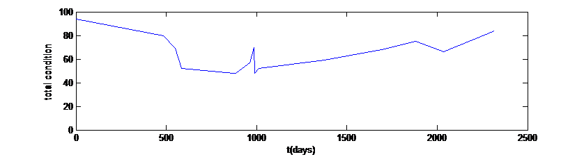Figure 5 Condition curve

At first, transformer condition has high value, as time passes, it decreases due to the degradation process. The degradation process produces gases, acid, water, which accelerate the degradation process.

There is a sudden increase in condition and then followed by a sudden decrease, this is probably caused by the maintenance process and the setting process after maintenance. After maintenance, the condition began to increase with small gradient.

The gradient of condition is shown in Figure 6.

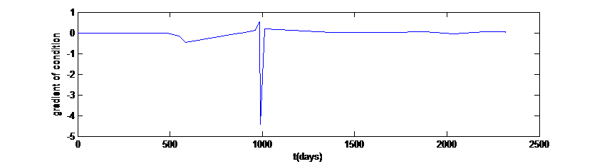Figure 6 Gradient of condition

The gradient of condition depends on condition. In general, it is relatively stable. There is a sudden decrease at day 990 and then followed by sudden increase.

The observation table is shown in Table 29.

Table 29 Observation table

t (days)	cond	gradient	SC	SG	NKPD
					HW	HL
0	94	0.0000	1	0	1	1
486	80	-0.0305	1	0	1	1
551	69	-0.1709	1	1	0	1
586	52	-0.4762	1	1	1	0
873	48	-0.0129	0	0	1	1
884	48	0.0000	0	0	1	1
961	57	0.1203	1	1	1	0
985	70	0.5401	1	1	0	1
990	48	-4.4444	0	1	1	0
1011	52	0.1764	1	1	1	0
1374	59	0.0204	1	0	1	1
1692	68	0.0277	1	0	1	1
1882	76	0.0390	1	0	1	1
2034	66	-0.0624	1	1	1	1
2203	77	0.0657	1	1	1	1
2315	85	0.0661	1	1	1	1
2316	85	0.0000	1	0	1	1

Where:

• Cond: condition of the transformer
• Gradient: condition change over time
• SC: cond, after compared to standard
• SG: gradient, after compared to standard

NKPD is knowledge of the system at each time of observation. To obtain knowledge growth, NKPD is fused with the previous NKPD, in this case, NKPD from the beginning of observation. This process produced NKPD over time (NKPDT)

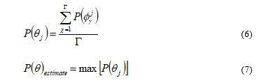
Knowledge growth is represented by NKPDT can be calculated using (6) and is shown in Table 30. Knowledge growth can also be represented using Figure 7.

Table 30 NKPDT

t (days)	NKPD
	HW	HL
0	0.5000	0.5000
486	0.5000	0.5000
551	0.3333	0.6667
586	0.2500	0.7500
873	0.3000	0.7000
884	0.3333	0.6667
961	0.2857	0.7143
985	0.2500	0.7500
990	0.3333	0.6667
1011	0.3000	0.7000
1374	0.3182	0.6818
1692	0.3333	0.6667
1882	0.3462	0.6538
2034	0.3214	0.6786
2203	0.3000	0.7000
2315	0.2813	0.7188
2316	0.2941	0.7059

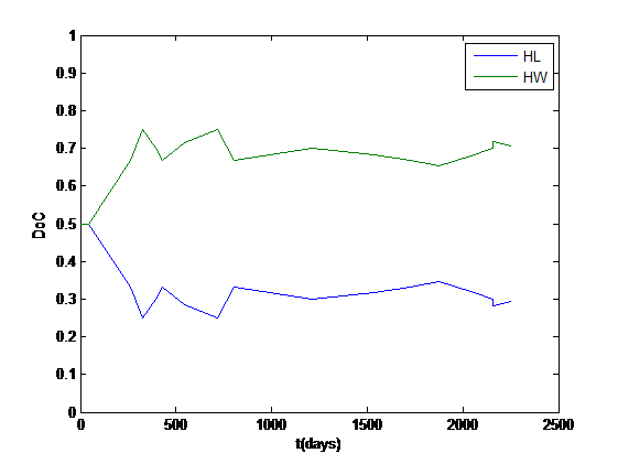Figure 7 Hypotheses/Knowledge growth

Where HL shows Hypothesis-Life and HW shows Hypothesis-Warning. Both hypotheses show the same value at the first observation. As time passes, HW increases, while HL decreases. It indicates that the transformer condition is in the limit and there are some changes in the gradient. The positive gradient shows maintenance, while negative condition shows degradation.

Spikes in Figure 7 shows there is an occurrence of a phenomenon indicating a hypothesis. In this case, there is a change in gradient of condition, making it in a warning condition. As gradient is dependent to condition, the hypothesis HW is dependent to HL as well.

5.       Concluding Remarks

A3S has successfully interpreted DGA data to identified fault based on the classified dataset. It has successfully identified not only the main fault, which has the most significant DoC. It has successfully identified the fault(s) occurred along with the main fault, which has less significant of DoC. This feature acts as the early warning system.

OMA3S has successfully interpreted transformer condition by fusing the parameter Condition (SC) and Gradient (SG) to produce Hypothesis-Life (HL) and Hypothesis-Warning (HW). HL and HW both are fused with the previous values to obtain knowledge growth.

In the next research, more parameters will be included and elaborated to increase accuracy. The number of hypothesis will be added as well to reduce the direct impact of the change of one hypothesis to the other when using only two hypotheses.

This algorithm will be implemented in form of a processor called cognitive processor. Using a special purposes processor will have advantages, such as energy efficiency and minimize disturbance caused by electromagnetic transmission.

Conflict of Interest

Hereby, The authors would like to declares that this article “Cognitive Artificial Intelligence Method for Interpreting Transformer Condition Based on Maintenance Data“ is an original work of our research group and has no conflict of interests.

Acknowledgment

The first author would like to appreciate Yokeu Wibisana for the maintenance data and Harry Gumilang of PLN for the discussion and information provided.

1. A. S. Ahmad and K. O. Bachri, “Cognitive artificial intelligence method for measuring transformer performance,” 2016 Future Technologies Conference (FTC), San Francisco, CA, 2016, pp. 67-73.
2. L. Po-Chun and G. Jyh-Cherng,”Research on Transforming Condition-Based Maintenance System using the Method of Fuzzy Comprehensive Evaluation”, World Academy of Science, Engineering and Technology, vol. 5, 2011
3. H. Gumilang, “Hydrolysis process in PLN P3BJB transformers as an effect of oil insulation oxidation,” 2012 IEEE International Conference on Condition Monitoring and Diagnosis, Bali, 2012, pp. 1147-1150.
4. A. D. W. Sumari, A. S. Ahmad, A. I. Wuryandari, J. Sembiring, “Brain Inspired Knowledge Growing System: Towards a True Cognitive Agent”, IJCSAI Vol. 2 Issue 1, 2012
5. K. O. Bachri, B. Anggoro, A. S. Ahmad, “Transformer Performance Calculation Using Information Fusion based on DGA Interpretation”, 2016 IEEE International Symposium on Electronics and Smart Devices (ISESD), Lembang, 2016.
6. Z. Qi, W. Zhongdong, and P. A. CROSSLEY, “Power Transformer End-of-life Modeling: Linking Statistical Approach with Physical Ageing Process”, CIRED Workshop, June 2010.
7. IEEE Guide for the Interpretation of Gases Generated in Oil-Immersed Transformers,” in IEEE Std C57.104-2008 (Revision of IEEE Std C57.104-1991) , vol., no., pp.1-36, Feb. 2 2009
8. IEEE Guide for Acceptance and Maintenance of Insulating Oil in Equipment,” in IEEE Std C57.106-2006 (Revision of IEEE Std C57.106-2002) , vol., no., pp.1-36, Dec. 6 2006.
9. M. Duvall, A. dePablo,”Interpretation of Gas-In-Oil Analysis Using New IEC Publication 60599 and IEC TC 10 Databases” IEEE Insulation Magazine, Vol. 17, No. 2, March/April 2001, Feature Article.

(Click to view)

(Click to view)

No. of Downloads Per Month

No. of Downloads Per Country