1. Introduction

This paper is an extension of work originally presented at the IEEE International Conference on Industrial Engineering and Engineering Management, Indonesia in December 2016 [1]. The positive feedback from the audience helped in writing a more detailed mathematical description of the growth functions. Furthermore, the energy density of Li-Ion cells was analysed and added to the case studies, because of its relevance in future automotive driveline systems. The summary section includes an overview of the technology assessment for this newly added energy storage technology. An extended conclusion shows the influence of the approach introduced on strategical Technology Management. The newly added outlook paragraph discusses the benefits of a fundamental figure-based approach in combination with data mining for strategic decision making in research and development departments. With the help of a reporting system and individually derived performance indicators the future possibilities of making the right decisions will rise. In a big data driven, rapidly growing digital environment, new fields of application in many engineering branches will appear for the integration of the method.

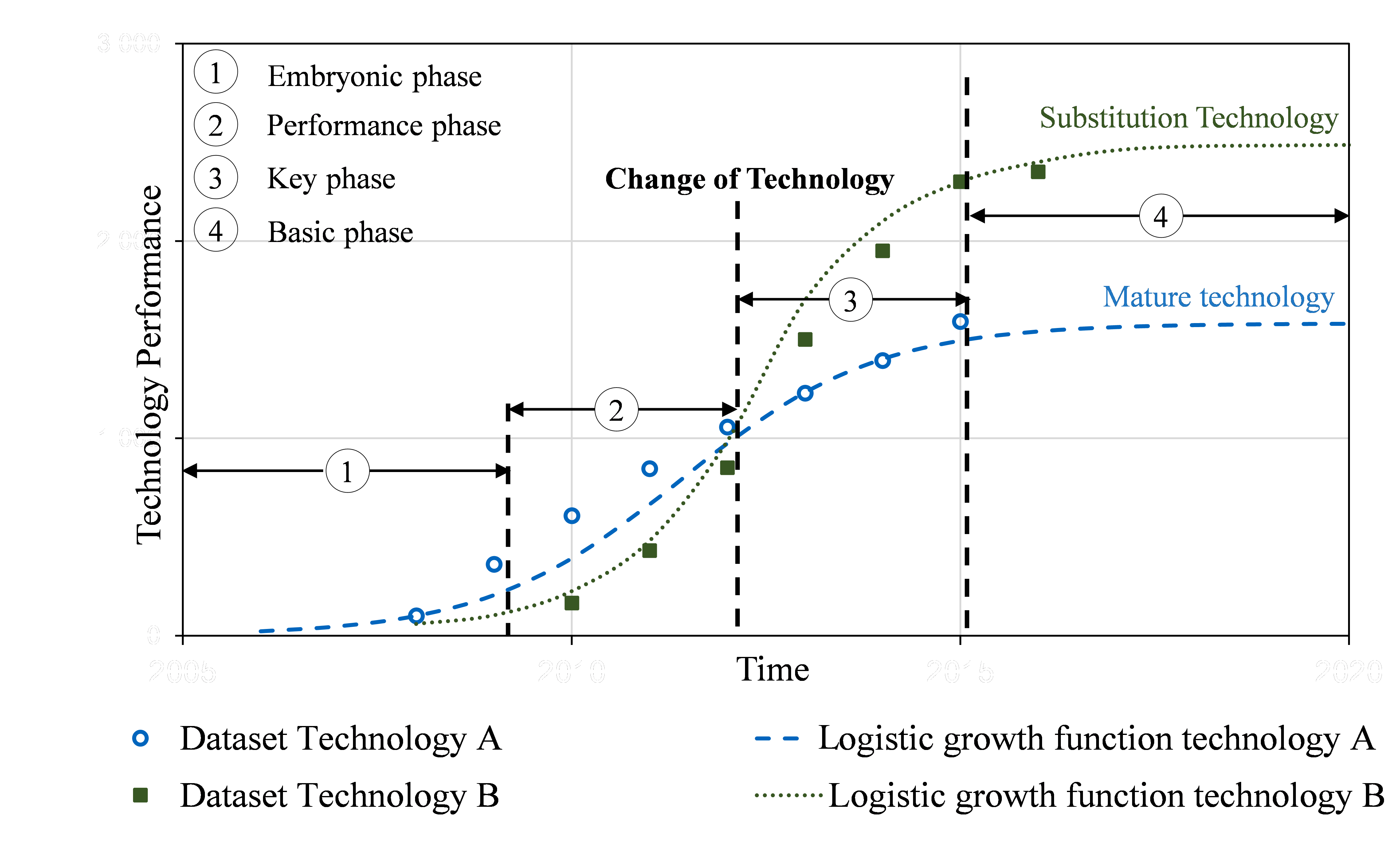Figure 1: S-curve model, Technology A is substituted by Technology B, the growth phases refer to Technology A [5].

Due to the rapid arrival of substitution technologies, companies are under growing pressure to make fast and sustainable decisions. In the past, even companies with market leader positions such as AOL, Kodak, Nokia and Grundig [2 ]have disappeared due to their reliance on outdated technology. According to methods such as the Gartner Hype Cycle and the technological lifecycle of Arthur D. Little [3], different stages of maturity describe the acceleration and deceleration of the achievable potential. The beginning and end of technological growth is qualitatively described by the S-curve model [4]. Figure 1 shows a qualitative example of technology substitution due to different growth phases. The objective of this paper is to forecast performance development and maximisation of the achievable potential. Therefore, logistic and exponential growth functions are used to quantify different growth patterns. This paper proposes a mathematical approach for technology forecasting and assessment.

2.       Methodology

Data collected from different branches of industry are analysed with the logistic growth function from [6] and [7] to determine the growth phases. If the technology is in its performance phase, the data are fitted with an exponential growth function from [8] to identify the future performance development. The exponential growth is similar to the performance phase of the S-curve model. The overall shape of the S-curve follows the logistic growth function. Figure 2 displays the overlay of the performance phases of a mature technology and a substitution technology that leads to extended exponential performance growth.

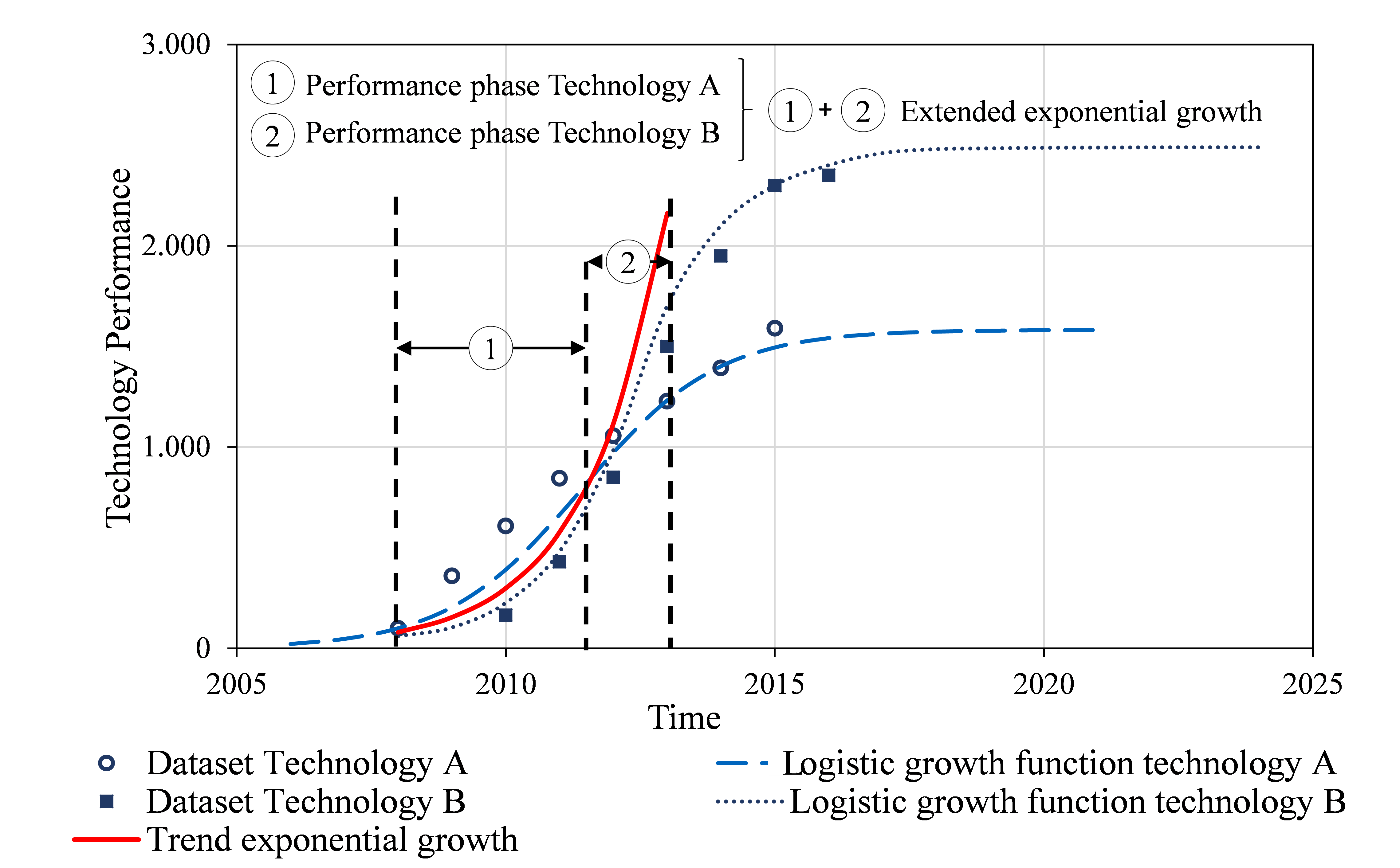Figure. 2: Extended performance phase by the overlap of two logistic growth functions.

2.1.  Mathematical description of logistic growth

Logistic growth is characterised by the growth coefficient r changing over time x, with y representing the performance of the technology and K the maximum value to be approximated, [6], [7]. Equation (1) gives the formula for the growth rate:

Figure 3: Slope of the technology growth rate

A positive slope in the growth rate leads to a continuous rise in technology performance. A negative slope of the growth rate corresponds to a slowdown in performance until the maximum value is approximated, Figure 3.

The logistic growth equation (2) follows from integrating (1) with the initial performance value y = y₀ at time x₀ = 0:

Figure 4: Determination of the growth coefficient r and the max. value K

The relative growth of the performance of a technology divided by the absolute performance y is linear relative to the absolute performance y. The linear equation can be derived from Figure 4.

Relative growth in relation to the absolute technology performance is described by the linear equation (3).

The maximum value K and the growth coefficient r, from (2), can be determined by solving the linear equation (3).

The growth rate r and the maximum value K follow from Equation (4):

Figure 5: Logistic growth function from Equation (2)

Given the maximum value K and the growth coefficient r, the logistic growth function from (2) is described completely (see Figure 5.)

2.2.  Mathematical description of exponential growth

As shown in Figure. 2 the sum of the performance phases of multiple logistic growth functions leads to the continuous exponential growth of the technology performance. The effect is valid for many market developments.

Exponential growth is characterised by the growth coefficient r, the starting technology performance y₀ in the embryonic phase and the time x shown in (7) and [8]:

In exponential regression analysis, the existing data y are compared with the values calculated from the exponential curve equation (7). Equation (7) is logarithmised in Equation (8) to apply the method of least squares to the performance phase of a technology, [9].

In the case of exponential regression analysis, Equation (8) is searched for, given the assumption that the sum of squares of the distances of the actual values y from the calculated  values has a minimum (method of least squares). The size V is described by equations (9) and (10) and has to be minimised for the number of data pairs, k.

Partially differentiating with respect to y₀:To determine the constants r and y₀ as two unknowns with two equations, (10) is modified and the partial derivatives are set to zero to obtain the minimum.

Partially differentiating with respect to r:

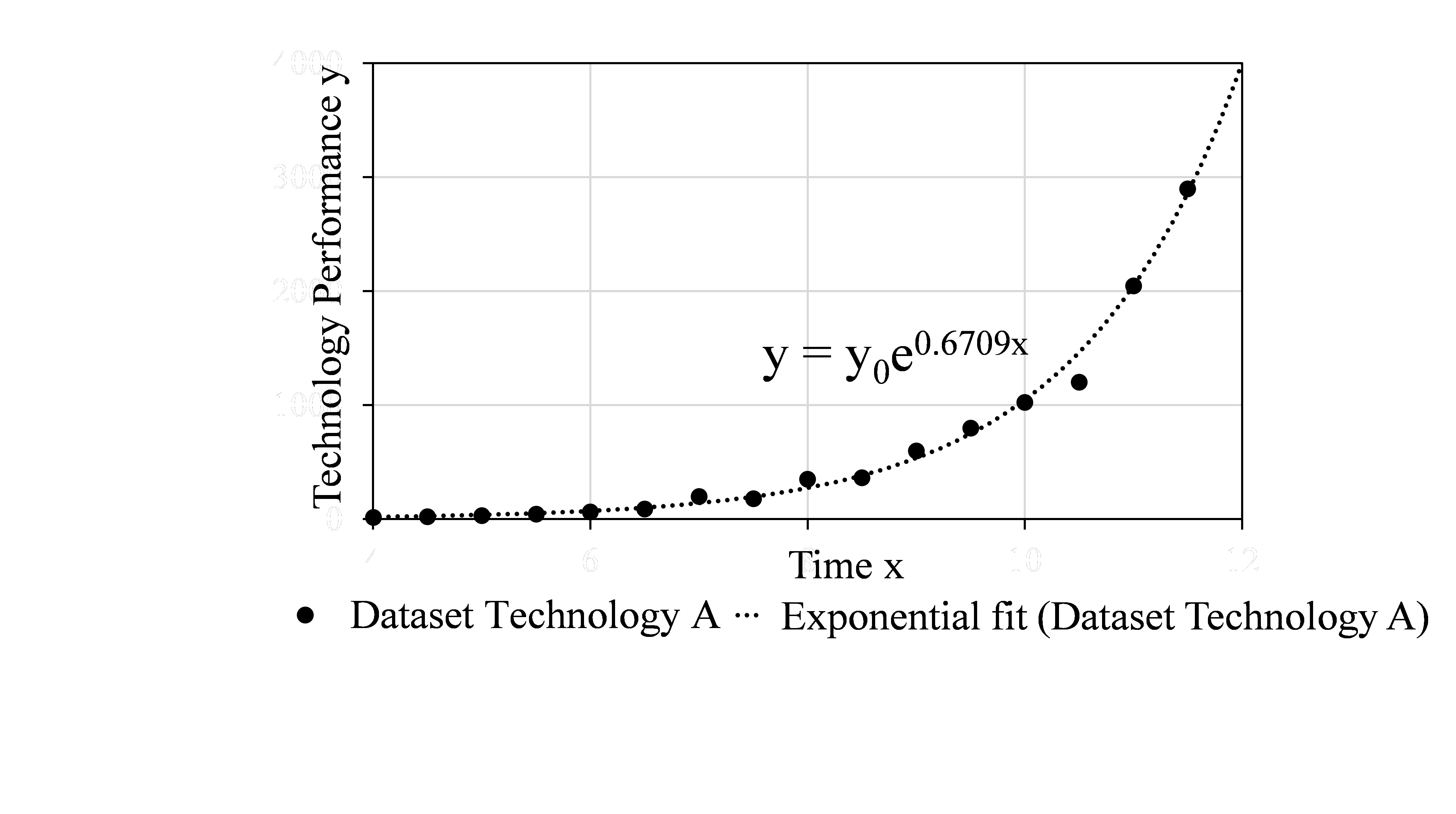Figure 6: Determination of the growth coefficient r, in the graph r =0.6709, which corresponds to an annual technology growth of 67.09%

In exponential regression analysis, the existing data y are compared with the calculated values  from the exponential curve equation (7). The method of least squares from [9] is applied to Equation (7) to find growth coefficient r during the performance phase, see Figure 6.

Given the growth coefficient r, the exponential growth function from (7) is described completely. The period during which the performance of technology doubles is calculated with the equations (19) and (20):

Doubling the performance implies y/y₀ = 2:

The fact that the natural logarithm of 2 equals 0.7 is the reason behind the 70-Rule, cf. (20), which is used in the automotive industry as a rule of thumb for rapid technology forecast and assessment.

3.       Analysed cases

In the example of Figure 6, the period of doubling of the technology performance is 70 divided by 67.09, resulting in 1.04 years.

In this section, the mathematical description of the technology performance is compared with actual data from technology undergoing continuous development. Five examples show the dependence of technology performance on growth functions. Each of the examples considered was individually analysed to identify logistic or exponential growth rates. The chosen examples are:

• Number of active Facebook users worldwide
• Tensile yield point of flat bar steel
• Number of transistors per unit area on integrated circuits
• Fuel efficiency per dimension of the VW Golf series
• Energy density of Li- Ion cells

3.1.  Number of active Facebook users worldwide

Table I gives the number of active Facebook users from 2008 to 2015 [10]. The data considered for the analysis begins in 2008, when Facebook launched French, German and Spanish versions, leading to a surge in users worldwide [11].

Table 1: Annual Number Of Active Facebook Users Worldwide, [10]

Active Facebook users worldwide
x	y
Quarter / Year	Number in millions
Q4 / 2008	100
Q4 / 2009	360
Q4 / 2010	608
Q4 / 2011	845
Q4 / 2012	1,056
Q4 / 2013	1,228
Q4 / 2014	1,393
Q4 / 2015	1,591

Figure 7 shows the determination of the growth coefficient r = 0.791 and the maximum value K = 1,582 using the linear equation (4).

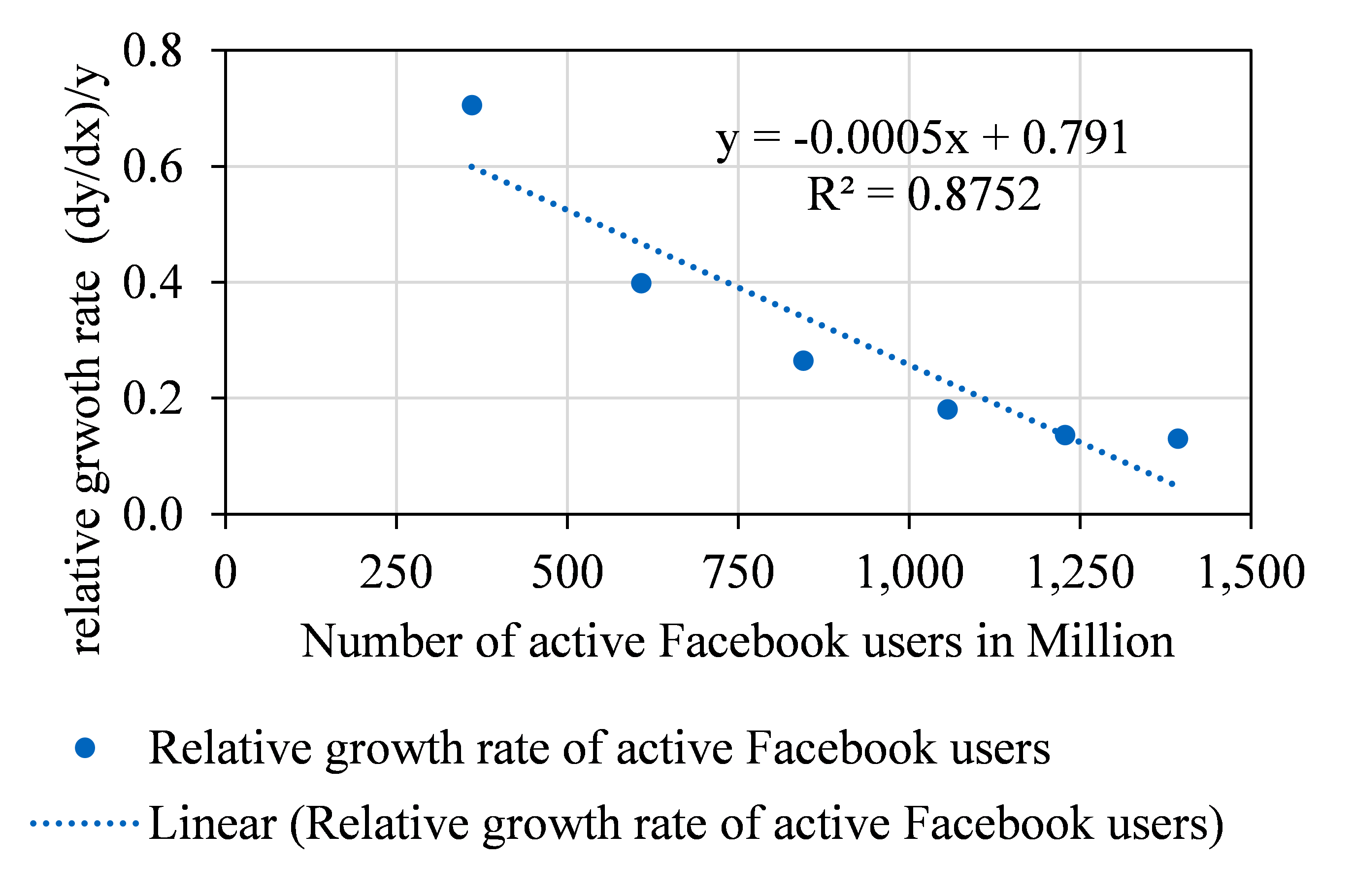Figure 7: Relative growth rate in relation to the absolute technology performance

Figure 8 displays the S-curve including the coefficients of the logistic growth from equation (2).

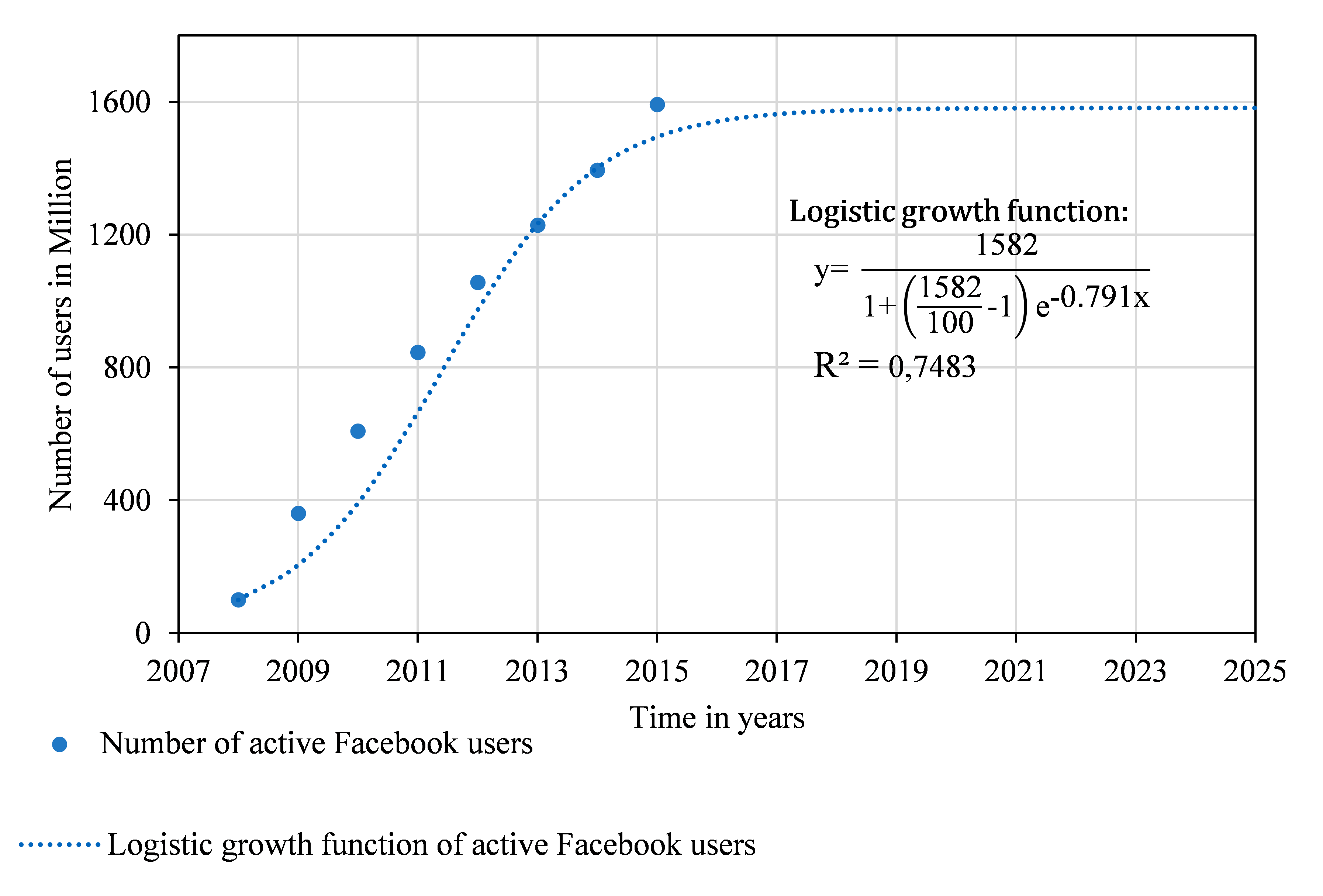Figure 8: Active Facebook users worldwide, described by logistic growth.

Conclusion: The relative growth rate of active Facebook users worldwide slowed down after the years 2009 and 2010. People without internet access represent the sleeping potential of the technology performance. Despite the slowdown in user growth, no substitute technology has been identified thus far.

3.2.  Tensile yield point of flat bar steel

The tensile yield point is a material parameter and designates the tension limit of non-permanent plastic deformation in the material. Table II gives an overview of the technological progression of the achievement potential.

Table 2: Tensile yield point of flat bar steel [12]

Tensile yield point of flat bar steel
x	y
Year	Tensile yield point in MPa
1926	355
1955	460
1965	690
1972	890
1980	960
1996	1,100
2013	1,200

Figure 9 shows the linear equation of the relative growth rate in relation to the absolute technology performance.

Solving the linear Equation with Equation (4), the values r and K are found to be equal to r = 0.0411, K = 1,500.

Figure 10 displays the logistic growth function adapted from r = 0.0411 to 0.03 due to a minimum set of data pairs relative to the period.

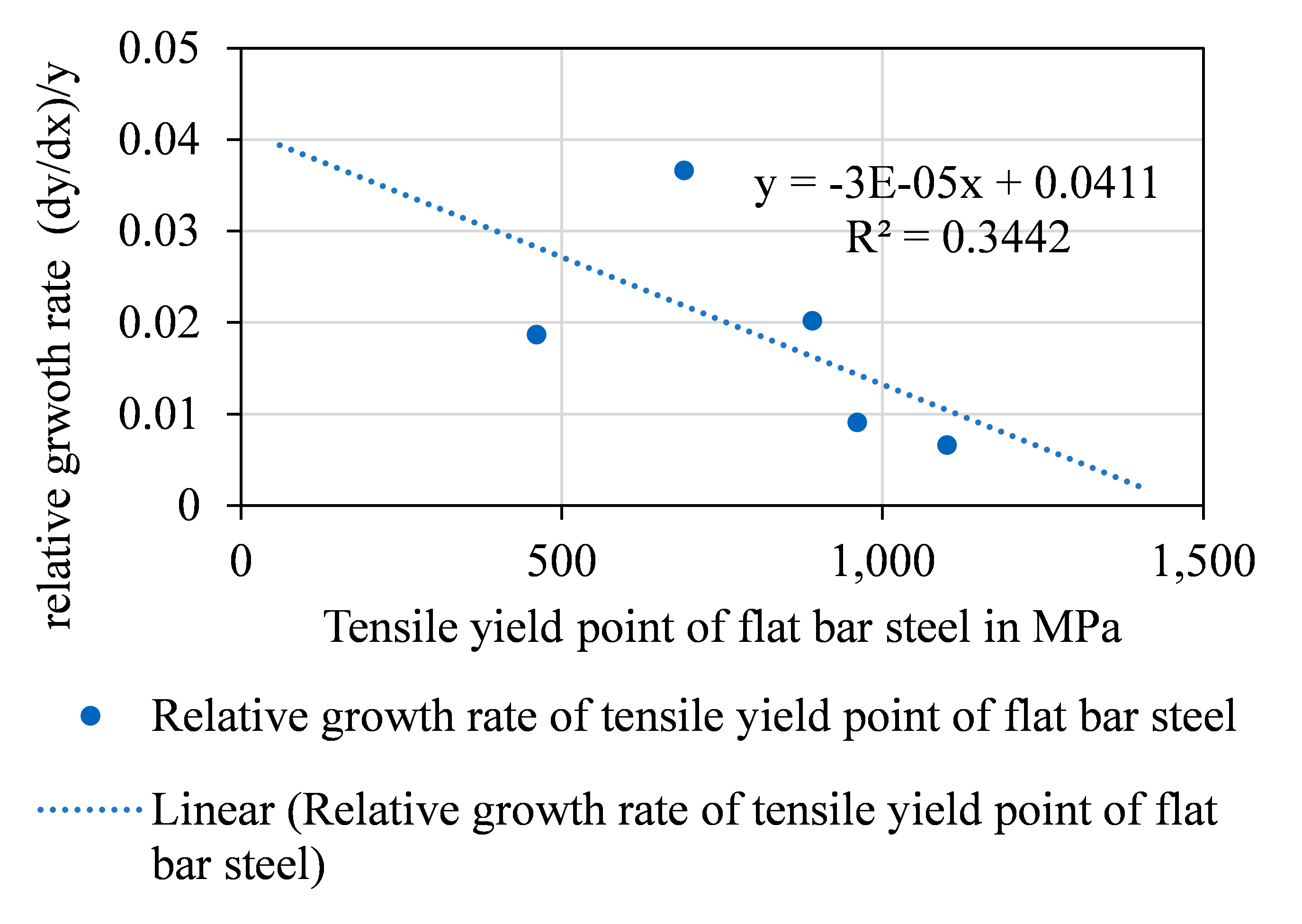Figure 9: Relative growth rate in relation to the absolute technology performance of flat bar steel

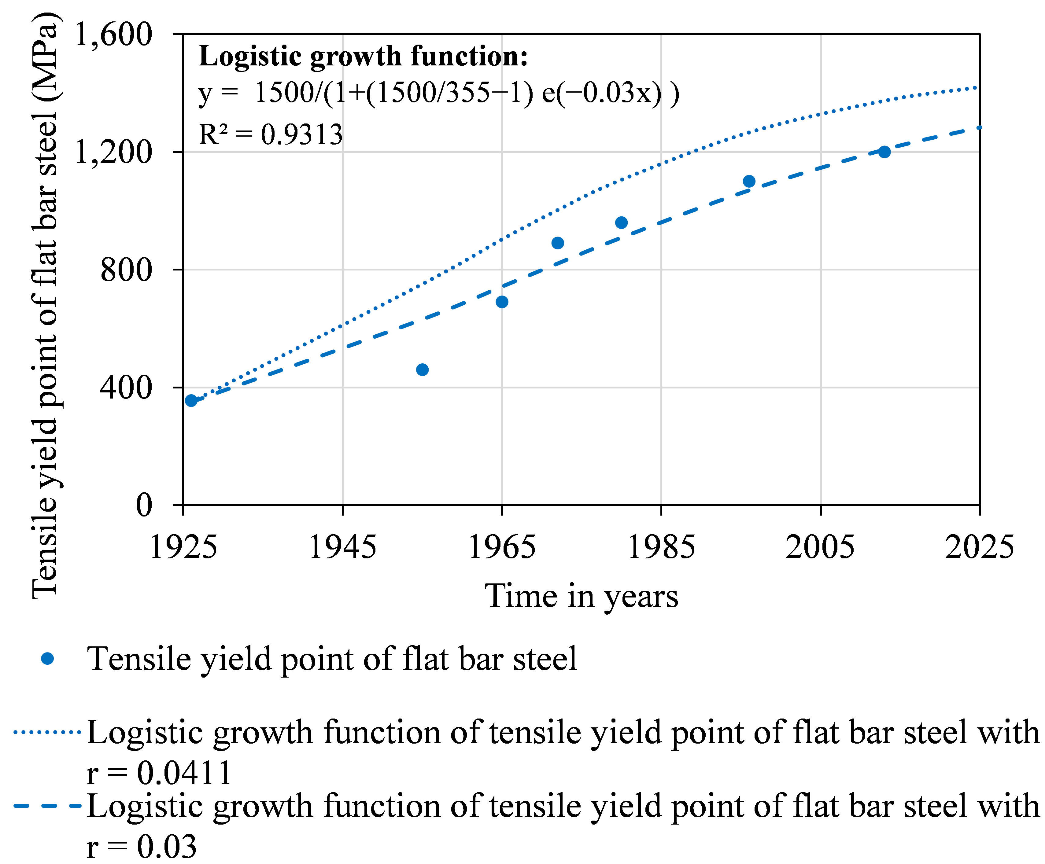Figure 10: Logistic growth function of the tensile yield point of flat bar steel with adapted growth rate from 0.0411 to 0.03.

Conclusion: The tensile yield point of flat bar steel from [12] has left the performance phase and is now in its key phase.

3.3.  Number of transistors per unit area on integrated chips

The number of transistors per unit area on integrated circuits is designated as the integration density, [13]. In 1965 Gordon Moore, Co-founder of Intel, predicted that the integration density will double every 12 to 24 months. This observation is known as Moore’s law. In [14] the executive Vice President of Intel William M. Holt, showed that there are leading technology options in the near future beyond complementary metal-oxide-semiconductors (CMOS) that can advance the exponential prediction of Gordon Moore. Table III depicts the integration density development.

Table 3: Overview of Integration density development on integrated chips [13]

Number of transistors per unit area on integrated circuits (integration density)
Processor	x	y
	Year	Integration density
Intel 4004	1971	2,300
Intel 8008	1972	3,500
Intel 8080	1974	4,500
Intel 8088	1979	29,000
Intel 80286	1982	134,000
Intel 80386	1985	275,000
Intel 80486	1989	1,180,235
Pentium	1993	3,100,000
AMD K5	1996	4,300,000
Pentium II	1997	7,500,000
Pentium 4	2000	42,000,000
AMD K8	2003	105,900,000
Itanium 2 with 9MB cache	2004	592,000,000
Cell	2006	241,000,000
Core 2 Duo	2006	291,000,000
Six core opteron 2400	2009	904,000,000
8-core Xeon nehalem-ex	2010	2,300,000,000
8-core Itanium Poulson	2012	3,100,000,000
Xbox One main SoC	2013	5,000,000,000
22-core Xeon Broadwell-E5	2016	7,200,000,000

Figure 11 shows that the mathematical determination of the growth coefficient r and the maximum value K with (4) is not possible. The reason is the continuous relative growth rate of the integration density, which has not slowed down over the years.

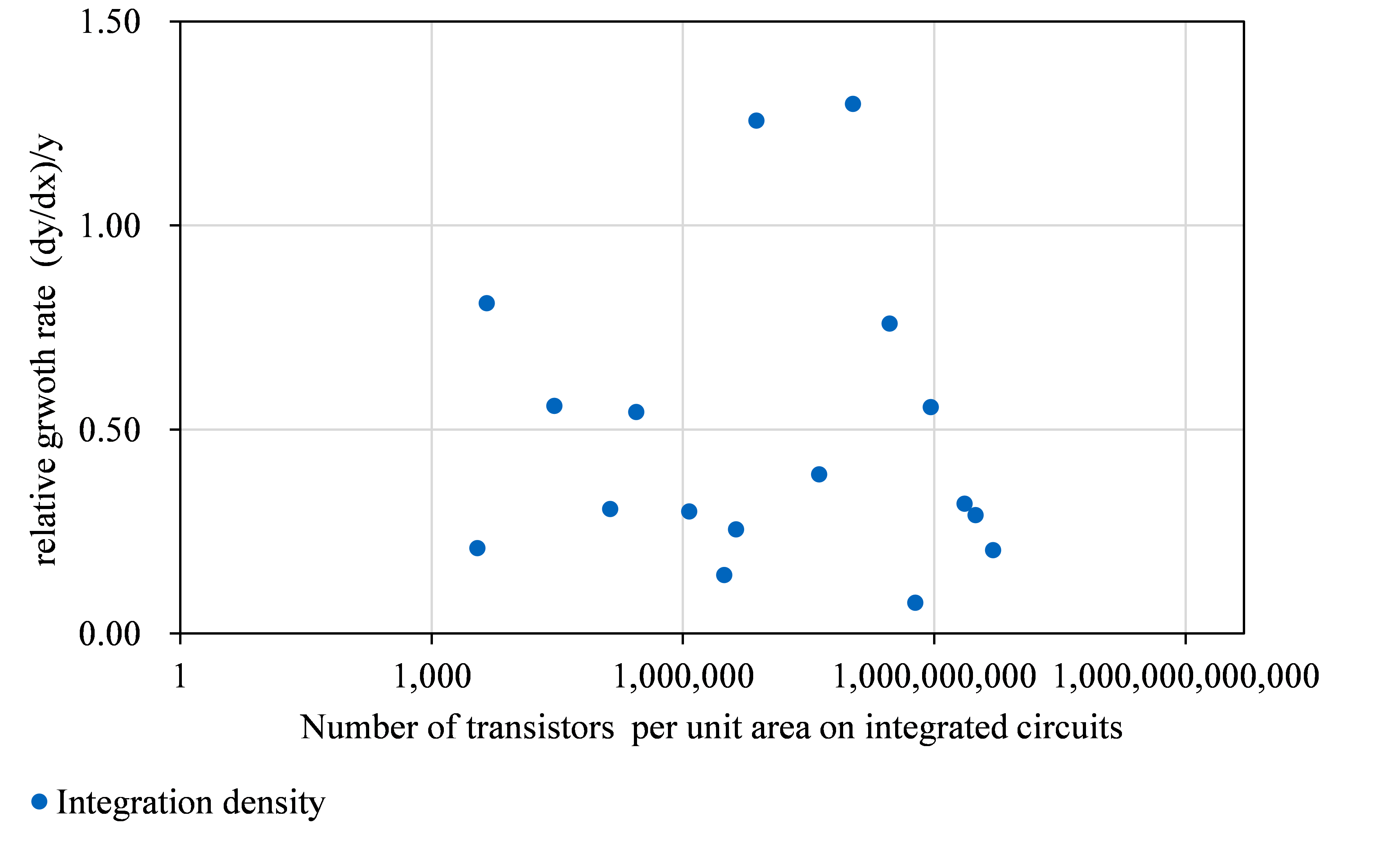Figure 11: Relative growth rate over a number of transistors per unit area on integrated circuits.

According to [14] the exponential growth of the integration density is based on the substitution of the process and the device technology. This leads to an extension of the performance phase. Figure 12 gives an overview of the innovations leading to the performance increase. The exponential fit uses the method of least squares from [9].

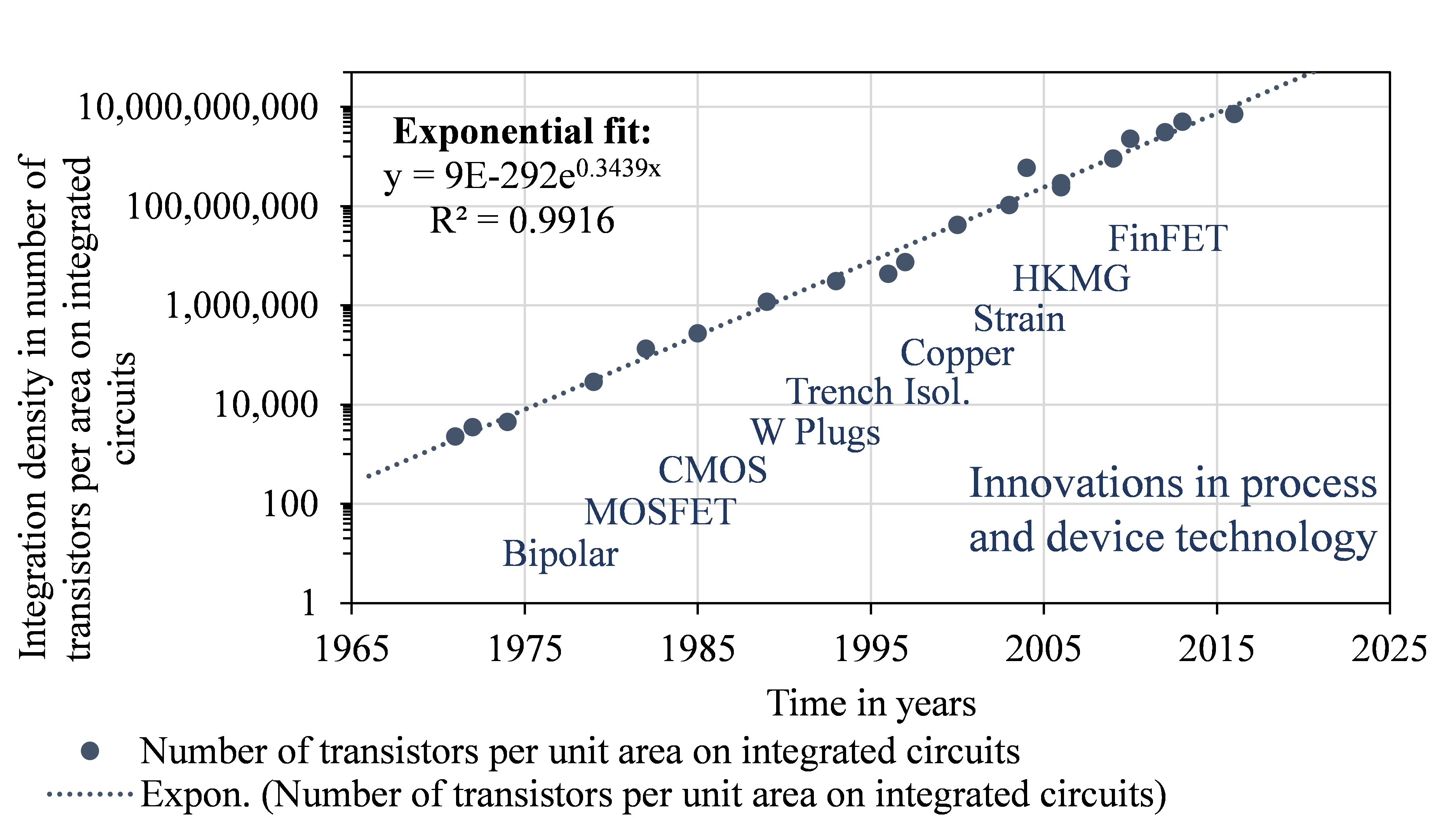Figure 12: Exponential growth of integration density on logarithmic scale

Conclusion: The trend demonstrated in Figure 12 shows the substitution of process and device technology leading to an extended performance phase. The time for doubling the number of transistors per unit area is around 2.04 years, taking into account an annual growth rate of 34.39 %. Moore’s prediction from 1965 is still valid.

3.4.  Fuel Efficiency per dimension of VW Golf series

The automotive industry faces new challenges such as carbon dioxide (CO₂) legislation in Europe with an upper limit of 95 g/km for every newly licensed passenger car from the beginning of 2020 [20]. In the United States, the Environmental Protection Agency (EPA) tightened the regulatory programme to 225 gram CO₂ per mile for passenger cars [21] this year. As a contrary trend, vehicle dimensions (length, width, height) are still increasing. Table V shows the fuel efficiency in kilometre per litre and the growing dimensions of the VW Golf series since 1976. That year, the VW Golf had its start of production (SOP) with its first diesel engine.

Table 4: Fuel efficiency Per vehicle dimensionS of VW Golf series I to Vii [22], [23], [24]

Fuel efficiency per vehicle dimension of VW Golf series (diesel engine)
Series	x							y
	Year of SOP	l/100 km	km/l	hp	ccm		l w h in m3		(km/l) m3
Golf I	1976	5	20.0	50	1,500		8.4		167
Golf II	1983	5	20.0	54	1,577		9.4		188
Golf III	1996	5	20.0	110	1,896		9.7		194
Golf IV	1997	4.9	20.4	110	1,896		10.4		211
Golf V	2007	4.5	22.2	105	1,896		11.0		244
Golf VI	2009	4.1	24.4	105	1,598		11.0		269
Golf VII	2012	3.8	26.3	105	1,598		11.1		292

Figure 13 depicts the relative growth rate over the fuel efficiency per vehicle dimension of the VW Golf series. Determination of the growth coefficient r and the maximum value K is not possible due to the positive gradient of the linear equation (4).

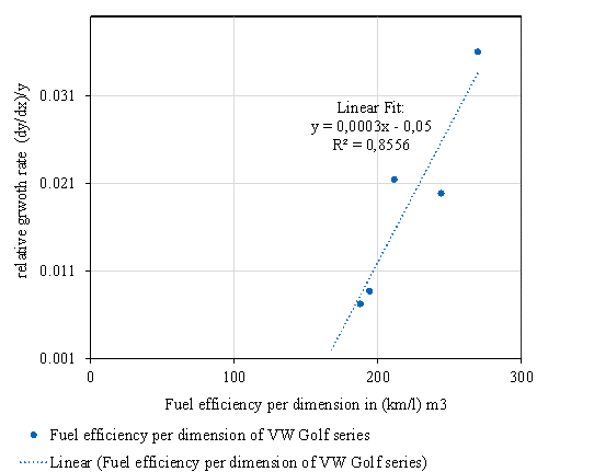Figure 13: Relative growth rate over fuel efficiency per vehicle dimension of VW Golf series

Figure 14 displays the exponential growth of the fuel efficiency per dimension. The coefficient of determination shows a correspondence of R² = 0.9062.

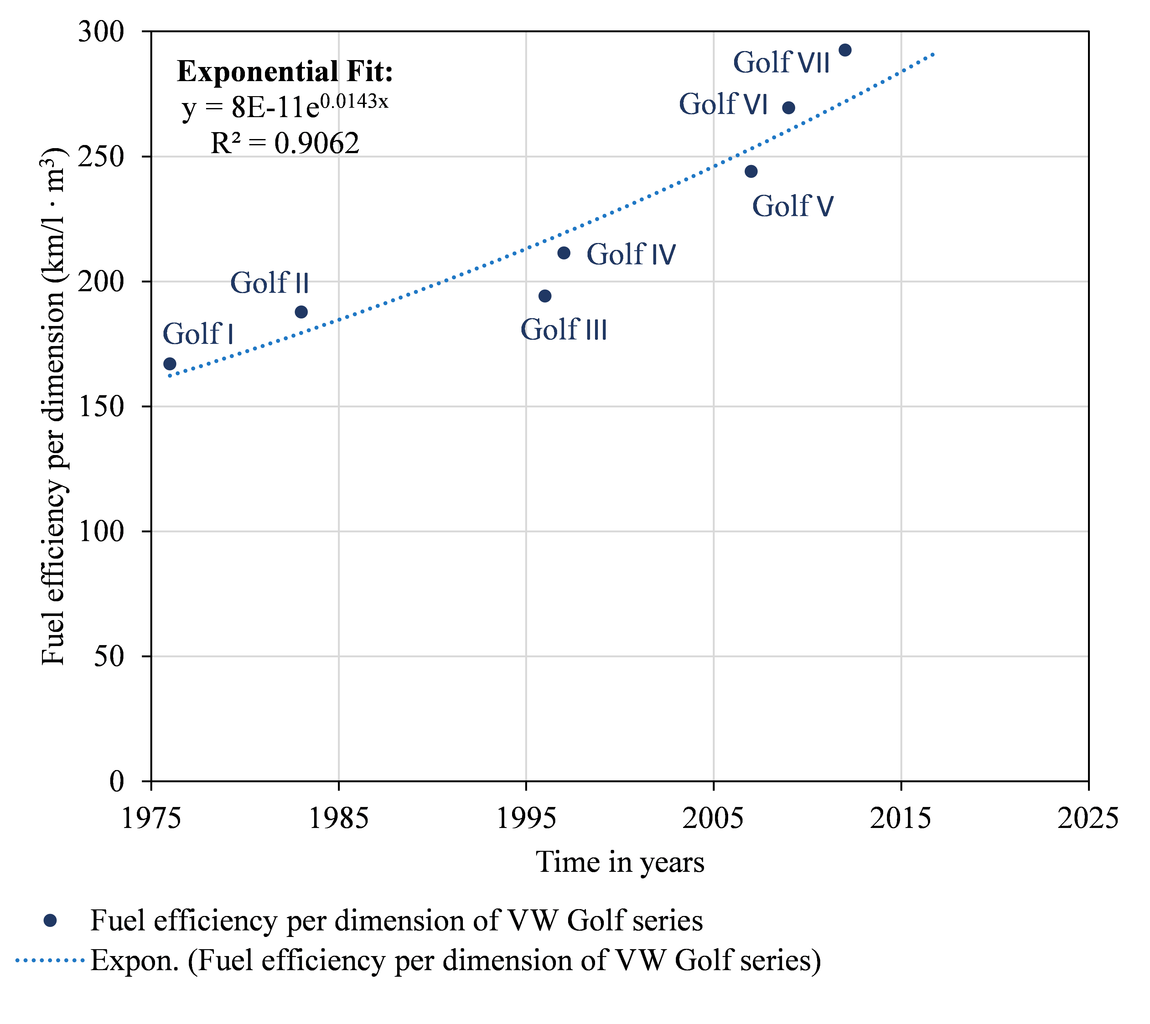Figure 14: Exponential growth of fuel efficiency per vehicle dimension of VW Golf series.

Conclusion: The fuel efficiency per vehicle dimension of the VW Golf series is exponentially increasing. The fuel efficiency of successive generations of vehicles has improved despite the increasing vehicle dimensions (length, width and height). The substitution of technologies in each vehicle generation has caused this effect, leading to the extension of the performance phase. The exponential annual growth rate determined amounts to 1.43 %. The 70 rule predicts a doubling of performance in 48.95 years.

3.5.  Energy density of Li-Ion cells

Over the next ten years, Li-Ion cells will not be only used in stationary and portable applications. According to [20], about 50 % to 70 % will be used in electro-mobility.

Table 5: Energy density of Li-ion cells with 18650 format [21], [22], [23] and [24]

Energy Density of LI-Ion cells
x	y
Year	Density in Wh/kg
1992	100
1996	110
1998	130
2000	140
2001	150
2002	160
2004	180
2005	200
2009	210
2010	230
2012	270

Figure 15 displays the relative growth of Li-Ion cells compared to technology performance in Wh/kg. The linear equation from (4) cannot be solved, as the relative growth rate does not slow down, while the growth coefficient r for logistic growth and the maximum value are not identified. The reason is the ongoing exponential growth.

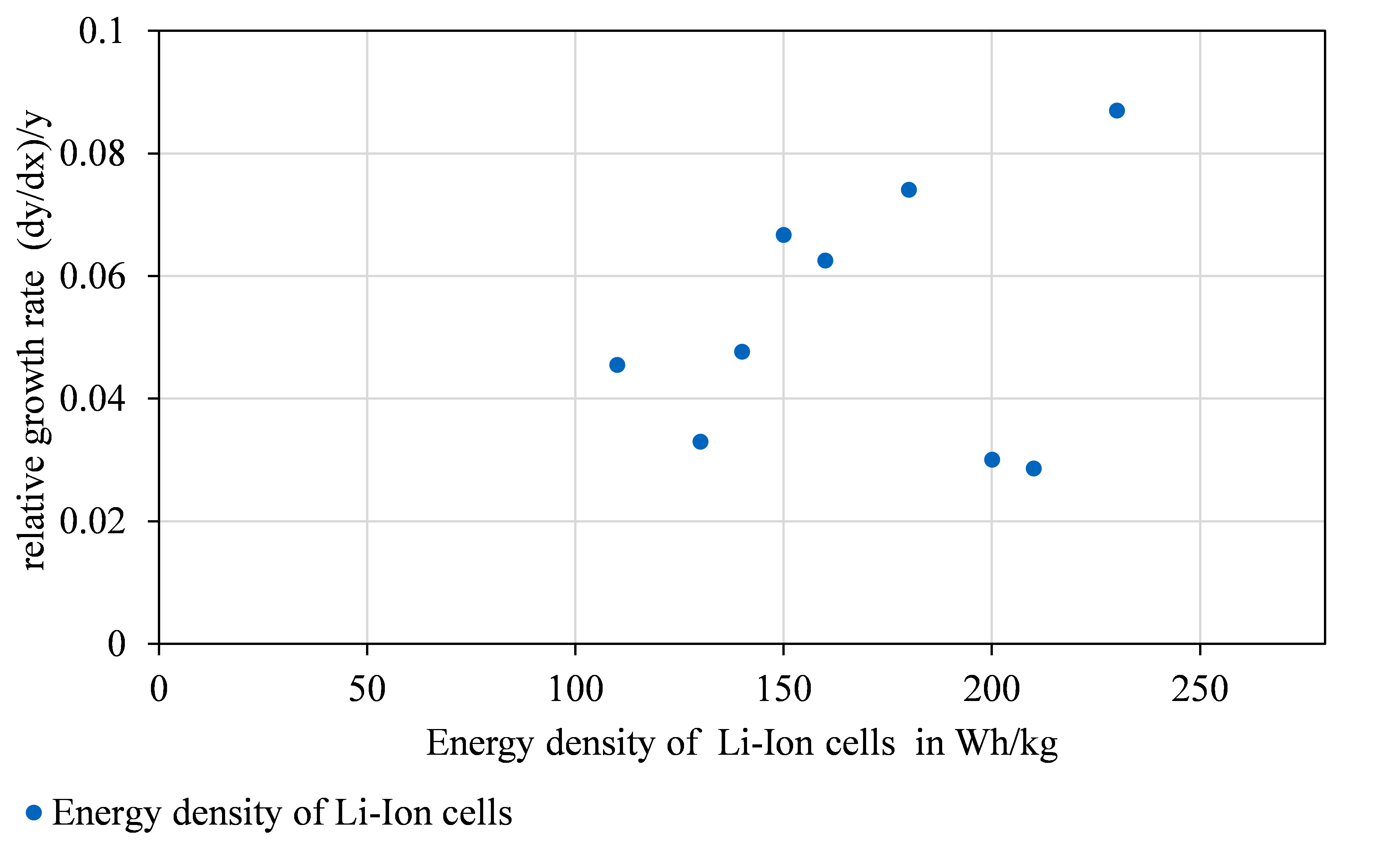Figure 15: Relative growth rate over energy density of Li-Ion cells

In Fig 16, the exponential fit shows a correspondence of 0.976 for the coefficient of determination R². Data points were matched with the names of cells from Sanyo/Panasonic.

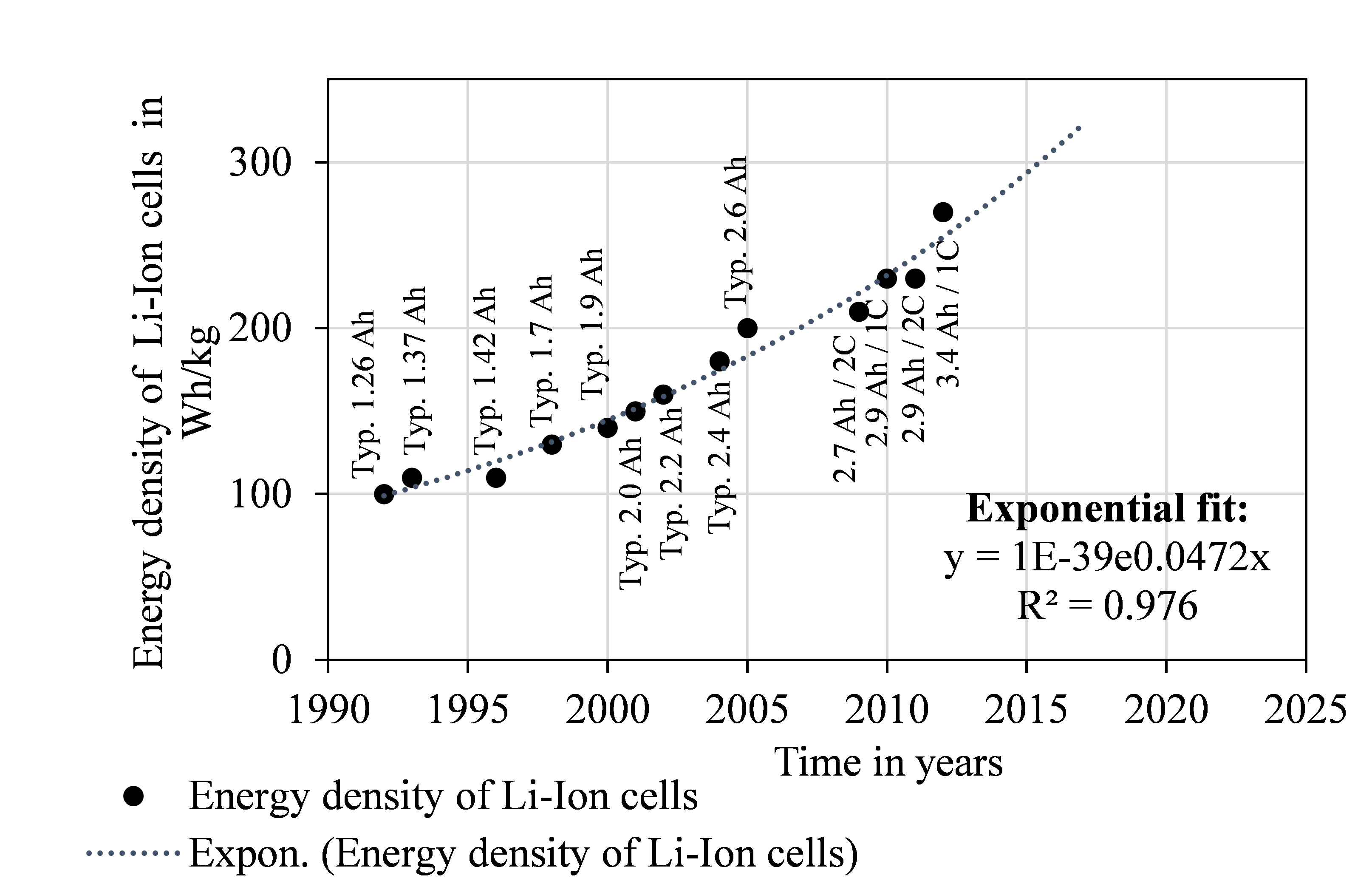Fig 16: Exponential growth of energy density of Li-Ion cells.

Conclusion: The energy density of Li-Ion cells is still in its performance phase. The substitution of the material composition of anode, cathode or separator leads to the extension of the exponential performance. The ongoing exponential growth has an annual growth rate of 4.72 %. Using the 70 rule, a performance doubling of the energy density in Li-Ion cells can be expected in 14.83 years. The Fraunhofer Institute for System and Innovation Research predicts that post-Li-Ion technology can reach a performance of up to 500 Wh/kg on the level of individual cells [20].

4. Summary and Conclusion

In response to the rising demand of companies to make reliable decisions based on TM and technology road maps, this paper proposed a mathematical approach for technology forecasting and assessment. The benefit for academics and industry is a quantitative method for identifying the level of technology maturity. The mathematical description of achievement potential using the logistic growth function has been introduced and compared with the S-curve model. Table VI gives an overview of the analysed case studies.

Table 6: Overview of results

Overview of results
Technology	Phase in the S-curve model	Period of performance doubling in years
Facebook user	Key phase	–
Tensile yield point of flat bar steel	Key phase	–
Number of transistors per unit area on integrated chips	Performance phase	2.04
Fuel efficiency per dimension of VW Golf series	Performance phase	48.95
Energy density of Li-Ion cells	Performance phase	14.83

The 70 rule for deriving the period of performance doubling, is a method for forecasting the technological development in its performance phase. Both rules are applied to a series of example cases. The results clearly show that the key technologies such as the number of transistors per unit area on integrated chips, the fuel efficiency per dimension and the energy density of Li-Ion cells are still growing exponentially.

5.        Outlook

Further investigation and discussion is needed to clarify whether integrating other relevant aspects that influence the technology performance forecast is meaningful. Firstly, an analysis must clarify which aspects can be considered as relevant for technological growth besides improvements in process and device technology: For instance, it is generally assumed that interdependencies exist between the improvement of the growth rate and aspects such as the financial environment and its characteristics such as resources, organisational structure and corporate culture. Secondly, the renewal time, during which the technology performance improves, must be measured precisely. It influences the shape of the S-curve model and can lead to transitions between the technological growth phases. Further possibilities, such as data mining and deriving key indicators for research and development topics, e.g. more precise online map data [25], lead to well-grounded decisions in strategic technology management. Technology road maps based on fundamental figures will be more successful in the long run. One of the next steps is the integration of automated search algorithms to gain a larger database for more accurate predictions of growth rates. An approach based on big data can help to gather more information over a shorter period. The future management of research and development will lead to a new dimension of decision-making tools.

Contributions

Special thanks go to Mr. Claudio Sutter, who helped to collect raw data for further investigation into technological growth during his master’s thesis in 2015.

Acknowledgement

This work was presented at the IEEE 2016 International Conference on Industrial Engineering and Engineering Management (IEEM16)

1. M. Fries, M. Lienkamp: “Technology Assessment Based on Growth Functions for Prediction of Future Development Trends and the Maximum Achievable Potential”, in IEEE Proceedings of 2016 International Conference on Industrial Engineering and Engineering Management, Indonesia, 2016. https://doi.org/10.1109/IEEM.2016.7798140
2. J. Höhmann, “New tools for strategists,” Harvard Business Manager Germany, vol. 6/2014, June 2014.
3. M. Steinert, L. Leifer, “Scrutinizing Gartner’s Hype Cycle Approach”, in IEEE Proccedings of Technology Management for Global Economic Growth, 2010.
4. G. Schuh, D. Guo and M. Wellensiek, “Approach for the Measurement of Technology Management Performance and Value”, in IEEE Proceedings of Portland International Conference on Management of Engineering and Technology, 2013.
5. G. Schuh, S. Klappert, Technology Management – Handbook Production and Management 2. Berlin, Heidelberg: Springer Verlag, 2011, pp.43 ff.
6. P. Blanchard, P. L. Devaney, G. R. Hall, Differential Equations. Boston, Cengage Learning, 2012.
7. P. Blanchard, P. Cummings: Course Math226.1x Introduction to Differential Equations. Module 1, Video 6 & 7. Boston University, https://courses.edx.org, last call 26.04.2015.
8. T. Wihler, Mathematics for Biology, Mathematical Institute, University of Bern, 2009, pp. 50-52.
9. University of Leipzig, “Regression analysis”, Informatics. http://www.stksachs.uni-leipzig.de/tl_files/media/pdf/lehrbuecher/informatik/Regressionsanalyse.pdf, last call 01.06.2016.
10. Internet Live Stats, Facebook active users, http://www.internetlivestats.com/watch/facebook-users, statistics analysed from statista.com, last call 10.06.2016.
11. M. Musgrove, “Facebook passes MySpace with global boost”, The Washington Post – Technology, June 2008.
12. Salzgitter Flachstahl GmbH, “Moderne Stahlvielfalt mit Blickpunkt Zukunft was die Automobilindustrie erwarten darf” (in German). Hannover Messe, 2013.
13. T. Häberlein, Computer Engineering. Wiesbaden: Vieweg + Teubner Verlag, 2011, pp. 2-5.
14. W. M. Holt, “Moore’s law: A Path Going Forward”, in IEEE Proceedings of International Solid-Stat Circuits Conference, Februrary 2016.
15. European Parliament and Council of the European Union, “Setting emissions performance for standards for new passenger cars as part of the Community’s integrated approach to reduce CO2 emissions from light-duty vehicles”, Regulation (EC) No 443/2009, April 2009.
16. United States Environmental Protection Agency, “EPA and NHTSA finalize historic National Program to reduce Greenhouse Gases and Improve Fuel Economy for Cars Trucks”, https://www3.epa.gov/otaq/climate/regulations/420f10014.pdf, April 2010.
17. Autodata, “Volkswagen – Golf VII”, http://www.auto-data.net/de/?f=showCar&car_id=17891, last call 01/06/2016.
18. Autoscout24, “Golf – 2008 until today”, http://autokatalog.autoscout24.de/vw/golf-vi-2008-heute/, last call 01/06/2016.
19. Autobild, “The real Volkswagen – VW Golf II 1983 – 1991/92”, “http://www.autobild.de/artikel/vw-golf-ii-1983-1991-92–44133.html, last call 01/06/2016
20. Fraunhofer Institute of System and Innovation Research, Roadmap energy storage for electromobility 2030, December 2015.
21. A. Kinoshita, “Development of Sanyo Li/Ion Batteries”, Sanyo Electric Co., Ltd, 2009.
22. SANYO: Cell Type UR18650ZTA, Specifications, June 2010
23. PANASONIC: Cell Type NCR18650PD, Specifications, February 2010, pp. 5-7.
24. PANASONIC: Cell Type NCR18650B, Specifications, January 2013, pp. 5-7.
25. M. Fries, M. Kruttschnitt, M. Lienkamp: ”Multi-Objective Optimization of a Long-Haul Truck Hybrid Operational Strategy And a Predictive Powertrain Control System”, in IEEE Proceedings of the 12th International Conference on Ecological Vehicles and Renewable Energies, Monaco Monte Carlo, 2017. https://doi.org/10.1109/EVER.2017.7935872

(Click to view)

(Click to view)