Skeletonization in Natural Image using Delaunay Triangulation
Skeletonization in Natural Image using Delaunay Triangulation
Volume 2, Issue 3, Page No 1013-1018, 2017
Author’s Name: Vicky Sintunata1, a), Terumasa Aoki1, 2
View Affiliations
1Tohoku University, Graduate School of Information Science, 980-8579, Japan
2Tohoku University, New Industry Creation Hatchery Center (NICHe), 980-8579, Japan
a)Author to whom correspondence should be addressed. E-mail: vicky@riec.tohoku.ac.jp
Adv. Sci. Technol. Eng. Syst. J. 2(3), 1013-1018 (2017); ![]() DOI: 10.25046/aj0203128
DOI: 10.25046/aj0203128
Keywords: Grey-scale skeletonization, Delaunay triangulation, Natural image, 2D skeleton

Export Citations
In this paper a novel approach to extract 2D skeleton information (skeletonization) from natural image is proposed. The work presented here is the extension of our previous paper presented at the International Sympsosium on Multimedia 2016. In the past work, a threshold based method is utilized. Here the algorithm is further improved by using a better edge points detection and skeleton extraction. Furthermore the proposed method is compared with the Skeleton Strength Map (SSM) and shows better result visually and numerically (F-measure comparison).
Received: 18 May 2017, Accepted: 15 June 2017, Published Online: 11 July 2017
1 Introduction
This paper is an extension of the work [1] originally presented at International Symposium on Multimedia 2016 (ISM’16). In this paper we provide a more detail and some improvement from the previous paper presented at ISM 2016.
Skeletonization is a process to extract the simplest, the most compact form of an object (skeleton) from 2D or 3D objects. Although mostly used in animation[2], skeleton information has also been used in symmetry detection [3], shape analysis [4], etc. Based on the input to the skeletonization, we can classify it into two types; 2D skeletonization and 3D skeletonization. In this paper, we are dealing with the first type, i.e. the 2D skeletonization or skeletonization from an image.
Corneat et al.[5] classify skeletonization into 4 classes, i.e. thinning and boundary propagation, distance field-based, geometric and general-field functions. While most of these approach works well, it only applies to the binary image. In order to get the binary image, of course one can use a foreground-background separation, but unfortunately foreground-background separation is still an open problem in image processing field. Another way to see the problem is that conventional approaches need a closed boundary information to extract the skeleton information. It holds when the object and the background information has a high contrast, but does not hold for object with a low contrast value with the
background (such as similar color and texture).
When the input image is not a binary image, the skeletonization is often referred as grey-scale skeletonization. Grey-scale skeletonization can be regarded as a relaxation of the conventional skeletonization. Instead of a binary image, the input to greyscale skeletonization is usually the brightness image (grey-scale image) or the color images. Skeleton is related closely to the symmetry information, therefore several authors are utilizing the symmetricity. You and Tang[6] proposed a method to detect the skeleton of characters using the wavelet. Widynski et al.[3] proposed a method based on particle filter approach. Levinshtein et al.[7] proposed a method based on superpixel segmentation and learned affinity function. In the last two methods, a supervised learning step is incorporated.
Du et al.[8] proposed a method based on a structure adaptive anisotropic filtering. The method is extracting the skeleton by updating the scale orientation and kernel of every pixel. The process is done iteratively including the update step therefore requiring a high computational cost. Another method is proposed by Li et al.[9] using a distance transform method [10]. By first extracting the edge information using Canny edge extraction algorithm and then calculating the inverted of the distance transform, this method can extract the skeleton of the object and its surrounding. To further increase the performance, a learned context model is utilized. Since this method relies on the distance transform, connected edge pixel is needed to some extend. It is important to note again here that while the connected edge pixel can be retrieved or extracted in an image where the object has high contrast, the opposite is not true. This condition results in a sparse or unconnected edge pixels in the image.
Most of the papers mentioned above has high computational cost or need a learning step in one of their method. In this paper we tried to solve the grey-scale skeletonization without a learning step. Furthermore the proposal can be used to relax the unconnected (sparse) boundary pixel condition. The rest of the paper is as follows: in section 2 the more detail explanation of the proposed method is presented. In section 3 some examples of the result and discussion will be presented. Finally section 4 will conclude this paper.
2 Proposed Method
The general framework for the proposed method can be seen in Figure 1. There are three major steps in the method: boundary points extraction, skeleton extraction and pruning step.
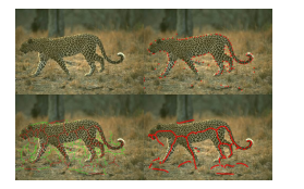 Figure 1: Proposed Method Framework. Upper-left: input; Upper-right: edge points extraction; Lower-left: skeleton extraction; Lower-right: pruning
2.1 Boundary Points Extraction
The method starts by making a grid of the input image and finding the edge points inside each grid. This edge points are selected by choosing the highest intensity among the pixels inside the grid. The question is then how are we suppose to find these edge points. It is very common to get the edge information from the gradient of the image. The higher the intensity of the gradient image is, the higher the probability it is considered to be the boundary object. Instead of using Canny edge detection which relies on the brightness image only, we calculate the edge (or gradient) information from both the brightness image and the color images.
First, the input image is converted into CIE color space and then split to each corresponding channels (i.e. brightness or luminance (L*) and two color channels (u* and v*)). Let ec(i,j) denotes the value of the gradient image at channel c (c ∈ L*, u*, v*) at (i,j) position. The value of ec(i,j) is calculated from the standard deviation of a pixel at (i,j) with its surrounding (n×n patch) at its respective channels (1). The benefit of calculating the standard deviation is that textured object will have a higher deviation which results in an easier way to locate the boundary pixel between two different objects. Finally we can combine them by averaging the values of these edge images (2) at each pixel.
vut n−1
Σa,b2=−n−21(xc(i +a,j +b)−x¯)2
ec(i,j) = σi,j,n = n2 (1)
e (2)
Since we are only interested on the boundary of the object, we can further reduce the texture effect by redoing the previous step onto the combined image (generated from 2). This will reduce the texture inside the object, but will also make the boundary of the object to lies inside a ”valley”. This can be avoided by applying the resulting image with the Laplacian operator. Let IL be the image after applying the Laplacian operator. IL will then be convoluted with the standard deviation image of the combined image, to construct the final edge image. Figure 2 shows the example of this approach.
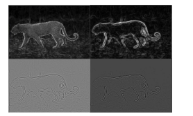 Figure 2: Edge Image Generation. Upper-left: combined image, Upper-right: Standard deviation image; Lower-left: Laplacian image; Lower-right: Final Edge image.
The edge points are then extracted from this edge image. Since we are selecting the edge points from the grid, there will be points which lie in the non-edge position. Filtering these points (candidate points) is done by using a method similar to a method proposed in [11,12]. The idea is very intuitive: at each pixel in the image, generate a patch and divide it into two halves along an orientation. At each section calculate its histogram (intensity, colors, etc.) and compare both of the sections. The higher the distance between the histograms (χ2 distance) the more likely the examined pixel to be an edge pixels.
Notice that we need to have an orientation at each candidate point. To approximate the orientation at each candidate point, the phase calculated from the difference of horizontal and vertical neighboring pixels of the edge image is used (Sobel operator). Let dx(i,j) and dy(i,j) denote the gradient in x and y direction respectively and θ(i,j) defined in (3), denotes the
phase at position (i,j). Let pθ(i,j) be the approximation of orientation in a candidate point with coordinate (i,j) and is defined by (4). Equation 4 means that the angle approximation is determined by the average of the phase surrounding the point. Finally the filtering is done by using the k-means (k = 2) algorithm with the histograms’ difference as features along with the intensity value at the corresponding pixel in the edge image.
y
θ(i,j) = (3)
pθ(i,j) = n2 a,b=−n−21 θ(i +a,j +b) (4)
Some of the points will lie very near with each other and it will affect the triangulation in the next step. Therefore a merging step is also applied to the filtered points, i.e. merging the points which lie near each other. The merged new position is calculated based on the average position of the merge points.
2.2 Skeleton Extraction
Skeleton extraction is done by first applying the Delaunay Triangulation to the edge points acquired in previous step. In order to do the skeleton extraction, a triangle grouping should be done. In [13,14] the authors classify triangles into 3 types: terminal triangle, junction triangle and sleeve triangle. The terminal triangle is defined as a triangle which has two outer contour as its edges. Junction triangle is defined as a triangle which does not have outer contour as its edges. Sleeve triangle is defined as a triangle which has only one outer contour as one of its edges. Note that in their application, which can be classified as the binary image skeletonization, the information regarding the outer edge is readily available. In our approach, we do not have that kind of information.
Note that in the previous step during clustering using k-means, we do have the idea to determine a point whether it belongs to the boundary points or non-boundary points based on its histogram distance feature. Therefore, we used this information to cluster the edge as follows. Let point mi be the middle point of the i-th edge. By applying the same approach as in section 2, i.e. orientation approximation and histogram calculation, we can determine point mi to be an edge point based on its (feature-) vector distance to the center points of each cluster. Another way to see this is, we are not recalculating the cluster centers since the cluster centers (which will determine whether a point is a boundary or non-boundary point) has already been calculated in the previous step, the evaluation of these edge points (m) can be done just by calculating the distance to the cluster centers. If dist(mi,Ck) is defined as the L2 distance between point mi and the k-th center, then point mi belongs to the the k-th cluster if it has the minimum distance compared to another cluster’s center.
In this case we can similarly define the triangles as in [13,14]. In sleeve triangle, two of its non-boundary m points will be connected together and no connection will be established in terminal triangle. Two types of junction triangles are defined: obtuse triangle and acute triangle. In case of acute triangle, an additional point (the center of triangle) will be added and every m points will be connected to this additional point. In obtuse triangle type, instead of generating an additional point, we connect the points on two of the edges of the largest angle to the point lying in front of the angle. See Figure 3 for visualization. Note that the yellow point (e.g. m1 in Figure 3.a) represents m belonging to the boundary cluster.
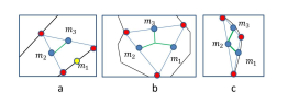 Figure 3: Three types of triangles: a. Sleeve; b. Acute Junction; c. Obtuse Junction .
Given an initial skeleton (point to point connection) from the previous step, the problem now is to determine which of the connection belongs to the same object. Let T denotes the set of pixels traversed by the skeleton’s edge (Figure 4). By calculating the mean pixel value of T we can get a set of feature vector (f) to represent the skeleton for the clustering algorithm (5). The subscript l denotes the type of image the pixel belongs to, i.e. color images, brightness image, etc. Figure 5 shows the result of the clustering algorithm. Note that since the contrast of the color images might be low for some images and resulting in a non-discriminative cluster, a contrast limited adaptive histogram equalization (CLAHE) is applied to the color images.
n
1 X
fl = Ti, Ti ∈ Tl (5) n
i=1
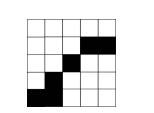 Figure 4: Pixels’ value traversed by the skeleton (black tile) will be included in the mean value calculation (5)
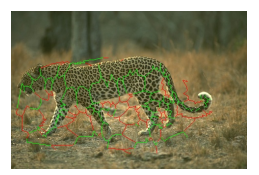 Figure 5: Example result of skeleton grouping
There is a possibility that the generated skeleton has a loop. In order to prevent such condition, loop removal step is applied. This is done by merging all the
position of the points belonging to that loop (Figure 6). If a loop consists of a smaller loop, only the largest loop is considered (Figure 7).
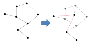 Figure 6: Loop removal step example. A new connection between the generated middle point c and remaining points are constructed.
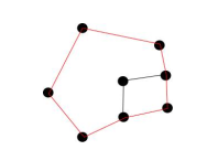 Figure 7: When there is a smaller loop inside a greater loop, only the outer loop will be considered (red lines)
2.3 Skeleton Pruning
Some might notice some redundant skeleton branches from Figure 5. Skeleton pruning is the step required to remove these branches. Borrowing the triangle types term, depending on the number of connection it has, skeleton points can be classified into three types: terminal, sleeve, and junction point. Terminal point means that the point only has one connection with another skeleton point. Sleeve point means that it has two connections with two other skeleton points. Junction point defines a point with more than two connections with other points. In this paper, skeleton branches are defined as the terminal points which
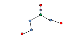 Figure 8: Colored points represent types of skeleton point. Red: terminal; Blue: sleeve: Green: junction
3 Experimental Result and Discussion
All experiments were done using a C++ language and OpenCV 2.4.9 library. There are several parameters which are fixed in this paper, i.e. the number of histogram bins is set to 16 and the size of the grid is set to 5 (refer to section 2.1). CIE Luv is used in this paper. Five images taken from the Berkeley dataset [15] were used for the experiment.
The results of the proposed method are then compared with a method based on [9]. Figure 9 shows the comparison, including the ground truth image generated by human observer. The first column is the ground truth skeleton image, the second column is the proposed method and the third column is skeleton generated based on [9]. Notice that although the proposed method did not generate the skeleton perfectly, it still represents the object in the image better than the method based on [9].
In order to further assess the result, F-measure of the ground truth and the methods were calculated
(6). The precision and recall is calculated following (7) and (8). The number of true positive (tp) is calculated by counting the number of pixel where both the ground truth (GT) image (with a σ = 1 allowance) and the generated skeleton image have the same value. σ here means that if the generated skeleton differs only slightly, i.e. still inside the allowance σ then it is still considered to be true positive and hence counted. Notice again that when comparing both the image to calculate the F-measure, skeleton image generated has binary color where the pixels will have a 1 (white colored) value if the pixel is not traversed by the skeleton edge and 0 (black colored) if it is traversed by the skeleton edge. For the false negative (fn), it is calculated as the number of pixel where it has a value of 1 in the ground truth image, but 0 in the skeleton im-
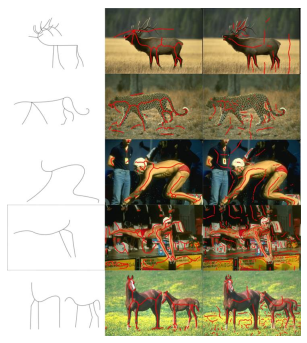 Figure 9: The skeleton is overlaid on top of the input image.
For visualization purpose, the skeleton is colored red.
|
P recision×Recall F = 2× P recision+Recall |
(6) |
|
tp P recision = tp +f p |
(7) |
|
tp Recall = tp +f n |
(8) |
Table 1: F-measure Results
| Image | Proposed | SSM[9] |
| Deer | 0.250 | 0.180 |
| Cheetah | 0.345 | 0.104 |
| Swimmer1 | 0.299 | 0.154 |
| Swimmer2 | 0.175 | 0.092 |
| Horse | 0.359 | 0.215 |
Although every image has its own best parameters, for general purpose, we try to find the parameter values which gave the best average F-measure from the test images. Four window sizes, which is used for histogram calculation, were tested (n = 7, 9, 11, and 15) along with the CLAHE limit parameter (l = 2 and 4). The result is shown in Figure 10. The x-axis is the combination parameters, i.e. (n,l). As shown in Figure 10 the combination of n = 9 and l = 4 has higher average F-measure among the other combinations.
Conflict of Interest The authors declare no conflict of interest.
- V.Sintunata, T.Aoki. ”Skeleton Extraction in Cluttered Image based on Delaunay Triangulation”, in International Symposium on Multimedia (ISM’16), 2016.
- I. Baran, J. Popovic´. ”Automatic Rigging and Animation of 3D Characters” ACM Trans. Graphics, 26(3), 72-1 – 72-8, 2007.
- N.Widynski, A.Moevus, M.Mignotte. ”Local Symmetry Detection in Natural Images Using a Particle Filtering Approach” IEEE Trans. Image Processing, 23(12), 5309-5322, 2014.
- X. Bai, L. J. Latecki. “Path Similarity Skeleton Graph Matching” IEEE Trans. PAMI, 30(7), 1282-1292, 2008.
- N.D.Cornea, D.Silver, P.Min. ”Curve-Skeleton Properties, Applications, and Algorithms” IEEE Trans. Visualization and Computer Graphics, 13(3), 530-548, 2007.
- X.You, T.Y.Tang. “Wavelet-based approach to character skeleton” IEEE Trans. Image Processing, 16(5), 1220-1231, 2007.
- A. Levinshtein, C. Sminchisescu, S. Dickinson. “Multiscale Symmetric Part Detection and Grouping” Int.J.Comput. Vis. 104(2), 117-134. 2013.
- X.Du, S.Zhu, J.Li. “Skeleton Extraction via Structure-Adaptive Anisotropic Filtering” in International Conference on Internet and Multimedia Computing and Service (ICIMCS’14), 2014.
- Q.Li, X.Bai, W.Y.Liu. “Skeletonization of Gray-Scale Image from Incomplete Boundaries” in International Conference on Image Processing (ICIP’08), 2008.
- L.J.Latecki, Q.Li, X.Bai, W.Y.Liu. “Skeletonization Using SSM of the Distance Transform” in International Conference on Image Processing (ICIP’07), 2007.
- D.R.Martin, C.Fowlkes, J.Malik. ”Learning to Detect Natural Image Boundaries Using Local Brightness, Color and Texture Cues” IEEE Trans. PAMI, 26(5), 530-549, 2004.
- M.Maire, P.Arbelaex, C.Fowlkes, J.Malik. ”Using Contours to Detect and Localize Junctions in Natural Images”in Conference on Computer Vision and Pattern Recognition, 2008.
- L.Prasad. “Rectification of the chordal axis transform and a new criterion for shape decomposition” Image and Vision Computing, 25, 1557-1571, 2007.
- T.Igarashi, S.Matsuoka, H.Tanaka. “Teddy: A Sketching Interface for 3D Freeform Design” ACM SIGGRAPH’99, 1999.
- Berkeley Dataset. https://www2.eecs.berkeley.edu/ Research/Projects/CS/vision/bsds/