1          Introduction

A brain computer interface (BCI) aims at detecting the presence of specific patterns in a person’s brain activity. These patterns relate to the user’s intention to control a device [1]. If such patterns are detected in the brain waves, then the BCI issues specific signals to control the device.

A brain computer interface (BCI) aims at detecting the presence of specific patterns in a person’s brain activity. These patterns relate to the user’s intention to control a device [1]. If such patterns are detected in the brain waves, then the BCI issues specific signals to control the device.

BCI systems can be classified into two categories: synchronous and self-paced [2]. In synchronous BCIs, the user controls the BCI output during specific short periods. Therefore, the user can only issue a control command when he/she is prompted to operate the system. Users of self-paced BCIs, on the other hand, ing which the user is not controlling the system are called No-Control (NC) states. During the NC states, the BCI system should be designed so it does not issue any control signal; otherwise a false positive output is produced.

Despite the much progress made in self-paced BCIs, they remain extremely challenging to design, compared with synchronous BCI systems. This is because (unlike the case of synchronous BCIs), a user of a self-paced BCI should be able to control the system at any time, but the BCI system does not have any knowledge about the onset of any control command.

To address this property of self-paced BCIs (i.e. the onset detection of intentional control), one of the following two approaches can be used. The first approach exploits the properties of the electroencephalogram (EEG) data to design more advanced classification and/or feature extraction techniques (the focus of this paper). For instance in [3] and [4] the authors have used more advanced classifiers to design self-paced BCI. The second approach takes advantage of other cognitive tasks to detect the onset of the intentional control. For instance in [5] the authors have used high pitch and siren-like sounds to facilitate distinguishing control tasks from no-control states. In [6] the authors have used a combination of motor imagery and P300 potential to design selfpaced BCIs.

The task of classifying brain signals in a self-paced BCI has been formulated as a sequential supervised learning problem [7]. In sequential learning, a sequence of observations and their corresponding labels are known, and the goal is to construct a classifier that predicts the sequence of the labels of a new sequence of observations.

The most popular way to obtain observation sequences for sequential supervised learning is to use a sliding window over the signal (these windows might overlap). This approach takes consecutive input windows of the brain signal (each of length w milliseconds), extracts features from each window and assigns a label to each window. The labels correspond to whether or not the user is issuing a command to operate the device. The sequence of the extracted feature vectors and their corresponding labels are used to train a classifier. For a new sequence, the trained classifier estimates the label of each window (i.e. the intention of the user).

The advantage of using the sliding window approach is that it converts the sequential supervised learning problem into a standard classification problem. Thus any classical supervised learning method can be used to solve the problem. The majority of the publications in the field have used this method to build different self-paced BCIs [8], [9], [10]. The disadvantage of the sliding window approach is that the sequential correlation of the labels of consecutive EEG windows is not exploited. Yet, the observations and the labels of nearby windows are usually related to each other. Thus there is a sequential correlation between adjacent EEG windows, and this knowledge could be used to improve the performance of the system.

In [11] the authors show that the brain goes through several well-defined internal state changes while the subject is carrying out a motor imagery mental task. Employing an algorithm that can model/exploit these state transitions can enhance the performance of the BCI. The class of sequence labeling algorithms are able to exploit the temporal structure of the EEG data. Among these algorithms, the most popular is the Hidden Markov Model (HMM) [12], which is a generative classifier. A generative classifier models the joint probability of observations and label sequences. Although the HMM classifier has been successful in synchronous BCIs, in [13] the authors concluded that the sliding window approach (i.e. using classical classifiers) is superior to HMM in self-paced BCIs. Due to intractability issues, HMMs assume the observations are independent given the states. This makes it difficult to incorporate knowledge about the structure of the EEG data into the model by extracting informative overlapping observations (the problem of over-counting evidence).

Another type of sequence labeling classifiers (besides HMM) are the discriminative ones. These classifiers directly maximize the conditional likelihood of the label sequence given the observations. These algorithms have yielded very promising results in the fields of natural language processing [14], and activity recognition [15] which are very similar in nature to the task of self-paced classification of BCI. The advantage of these models is that they give the user the freedom to extract many informative and overlapping features from the observation sequence. These features might be extracted from previous windows in the brain signal and can be correlated.

In [16], [17] and [18], the authors applied discriminative sequence labeling algorithms to self-paced BCIs, to classify different motor imagery tasks. In this paper, we use a discriminative sequence labeling algorithms to discriminate between NC and control states. The challenge here is that during the control states, i.e. while the subject is performing the mental task, a set of well-defined state changes occur. However, during the NC states, the subject can be in any mental state, therefore finding specific patterns in the EEG signal during NC states is extremely difficult. In other words, discriminating between two predetermined mental tasks (e.g. right hand versus left hand movement) is much easier than discriminating a predetermined mental task (e.g. left hand movement) from NC states.

Our contributions in this paper are two-fold. The first is a new discriminative sequence labeling classifier for self-paced BCIs. Our approach combines the power of one of the most popular discriminative sequence labeling classifiers (Conditional Random Field) to exploit the correlation in consecutive EEG windows. It also utilizes a neural network to extract high-level features from the observations. We call our classifier Neural Network Conditional Random Field (NNCRF). We compare its performance to those of Hidden Markov Models (HMM), and two of the most popular discriminative sequence labeling classifiers i.e. Conditional Random Field (CRF) [19] and Structural Support Vector Machines (SSVM) [20]. We also compare the performance of these discriminative sequence labeling classifiers with two popular classical classifiers i.e. Support Vector Machines (SVM) [21] and Logistic Regression classifiers [22]. Our second contribution is discussed in the latter part of the paper, where we propose an ensemble learning approach to further improve the accuracy of the BCI system. We use Bayesian optimization [23] to train several diverse classifiers on different parts of the BCI hyper-parameter space. We evaluate the performance of different algorithms using the data from the BCI competition IV [24] and SM2 [25] dataset, and show that our algorithm is considerably superior to the existing approaches in terms of the Area Under the Curve (AUC) of the BCI system.

In the rest of this paper, in section 2, we describe the feature function in discriminative sequence labeling classifiers. In section 3, we introduce our proposed sequence labeling classifier i.e. NNCRF. In section 4 we describe our ensemble classification approach. In section 5, we explain the datasets, and in sections 6 and 7, the results of different algorithms are compared.

2          Feature Function in Discriminative Sequence Labeling

For sequence labeling algorithms, we assume that each data sample in the training set consists of a sequence of observations, and its corresponding label sequence. Assuming the training set is {x_i,y_i}^N_i=1 where N is the number of training samples. x_i is the sequence of observations from K consecutive windows and y_i is the corresponding sequence of K labels. Every w milliseconds of the EEG creates a window. x_i is created by concatenating the observations from each of K consecutive windows i.e. x_i = [x_i1,…,x_ik,…,x_iK] and x_ik corresponds to the observations from the k^th window in the sequence number i. Likewise, y_i is created by concatenating the labels of each of these K consecutive windows i.e. y_i = [y_i1,…,y_ik,…,y_iK] and y_ik corresponds to the label of the k^th window in the sequence number i.

The discriminative sequence labeling algorithms have the advantage of enabling a set of features to be designed based on the structure of the data. Each feature is a function of the joint observations and their labels i.e. Φ : X × Y − > R, where X is the observation space, Y is the label space and R is the real space. In classical classification the feature vector is built based on the observations (X) only. However, here the idea is to extract features from the joint observations (X) and label (Y) spaces. In this way, a feature function Φ measures the joint compatibility of x (x_i) and y (y_i) ⁴. Although more complex types of features can be used, the feature functions we use here are inspired from first order HMMs.

The first feature function we used, is defined as

where I represents the indicator function, and Σ corresponds to the set of possible label values (i.e. NC states and movement states). The above feature function is based on Y only.

The second set of features forms a vector φ_k,1:L with L dimensions that captures the relation between the observation vector and the k^th label in the sequence. We are assuming the observation vector is of dimension L. Each element φ_k,l^σ of the vector φ_k,^σ _1:L is defined as

                               φk,lσ = xk,lI(yk = σ), σ ∈ Σ,                          (2)

where x_k,l is the l^th dimension of the observation vector.

The third type of features is defined as

where φ_k^σ₍¹_k^,σ₋²₁₎ captures the relation between the k^th and (k − 1)^th labels in the sequence.

3          Neural Network Conditional Random Fields

In this section we first describe the standard Conditional Random Field (CRF), then we describe Neural Network CRF. CRF is one of the most popular discriminative sequence labeling classifiers. In general the linear chain Conditional Random Field (CRF) classifier models the posterior distribution of the form

                                            J                K

                                            X         X

exp( λ_j Φj(y_k−1,y_k,x,k)) j=1 k=1

              Pr(Y |X) =  ,       (4)

Z(X)

where K is the sequence length, J is the number of features extracted from the joint observation labels pair, and Φ_j is the feature function. λ_js are the parameters of the model which are learned based on the training data. Z(x) is the normalization factor (partition function):

                                                      J                K

                          XX X                   X         X           _{0             0}

Z(X) = … exp( λ_j Φ_j(y_k−₁,y_k,x,k)). y₁0 y₂0 y_K0 j=1 k=1

(5)

To calculate the partition function we use forwardbackward algorithm which is a dynamic programming algorithm.

Using the above mentioned set of features (equations 1, 2 and 3) the posterior function will be of the

form

                                          K                                                          K

expX(byk +WyTk,1:Lxk)+XVyk−1,yk

Pr(y1:K|x1:K) =   k=1 k=2   ,

Z(X)

(6)

where b_yk, W_yk,1:L and V_yk−₁,y_k are the parameters of the posterior distribution and should be learned using the training dataset. The set of parameters b_yk,

W_yk,_1:L and V_yk,y_k−₁ capture the importance of the first, second and third type of features respectively.

To learn the optimal values of the parameters, we minimize the L₂ regularized negative log likelihood

N

X

min  −Log Pr(y_i|x_i)+Cλ^T λ,             (7) λ

i=1

where the vector λ consists of the parameters of the model (i.e. b_yk, W_yk,1:L and V_yk−₁,y_k), and C is the regularization coefficient. To find the optimal value of the parameters, we use stochastic gradient descent algorithm. As the loss function is convex, the gradient descent algorithm converges to the global optimum of the loss function.

For the inference i.e. assigning a sequence of labels to x_N+1, we assign the most probable sequence as the predicted labels i.e.

y_predicted = argmaxP (y|x_N+1).       (8) y

A Viterbi [12] like algorithm is used to find the most probable sequence of labels.

The linearity of the exponent term in CRF makes this classifier to have less expressive power compared to the classifiers that exploit kernels. A good approach that makes these algorithms more powerful is to pass the data through a feed-forward neural network before applying the CRF part. Neural networks transform the observation vector into high level features which are then used as the input to the CRF. As a result, the exponent term in CRF (i.e. the exponent term in equation 6) becomes non-linear because of the several layers of non-linear activation functions that have been applied on the observation vector [26] [27]. This combination of a neural network followed by a CRF forms our proposed classifier which we denote by

NNCRF (Neural Network Conditional Random Field).

The NNCRF can be viewed as a standard linear chain CRF that uses a high level representation of the observations. Therefore, the posterior function of NNCRF has the same form as in equation 6 except that the x_k terms are replaced with the h^M(x_k) term which represents the output of a feed-forward neural networks with M layers.

                                K                                                                                K

exp(X(byk +WyTk,1:Lh(M)(xk)yk)+XVyk−1,yk)

Pr(Y |X) = k=1    k=2                 .

Z(X)

(9)

The output of the (M)_th layer (h^(M)) is h(M)(xk) = tanh(b(M−1) +W (M−1)hM−1(xk)), (10) where b^(M−1) and W ^(M−1) are the weights of the (M − 1)^th layer, h^M−1(x_k) is the output of the (M − 1)_th layer of the neural network, and h⁰(x_k) = x_k. To avoid overfitting, the weights of the neural networks are the same for all observations x_k in a sequence i.e. the values of the weights do not depend on k.

Initialization of a neural networks is very crucial for this algorithm to converge to a good local optima. For initialization of the neural network, the value of each parameter is a sample taken from a uniform distribution U[−γ,+γ] where

√

6

γ = _p ,               (11) size(M)+size(M − 1)

where size(M) is the number of hidden units in the M^th layer of the neural networks.

The loss function is the same as the loss function of the standard CRF (Equation 7). The values of the parameters of the neural networks and of the CRF are jointly optimized using the back propagation algorithm. The learning rate of the stochastic gradient descent algorithm is adjusted using the bold driver approach. For inference the same algorithm as in standard linear chain CRF is used.

4          Ensemble of classifiers

In [28], the authors proposed an algorithm to customize the synchronous BCI based on the brain characteristics of each subject. Here, we adopt a similar approach to build an ensemble of classifiers for selfpaced BCIs based on the brain characteristics of each subject.

The brain characteristics of each subject are captured in the form of some hyper-parameters of the BCI system. Hyper-parameters are the parameters of the BCI system which are selected before feature extraction and classification. We use Bayesian optimization which is an iterative algorithm to propose the values of the hyper-parameters. The proposed values of the hyper-parameters are used to train different classifiers on different parts of the input space. Then, we combine the results of the trained classifiers, using averaging, to form the output of the ensemble classifier.

Bayesian optimization [23] [29] optimizes an objective function g(x) over some bounded set X. The objective function does not have a closed form expression and its derivative is unknown. A Bayesian optimization algorithm sequentially constructs a probabilistic model for g(x) and then uses this model to select a candidate for the optimization task. In our case, the objective function is the cross-validation accuracy of the classifier. The input to the Bayesian optimization algorithm consists of the values of the hyper-

parameters of the BCI system. Therefore the set X is the hyper-parameter space of the BCI system.

In this study, the hyper-parameter space of every classifier consists of the frequency ranges to filter the EEG signal, the selected channels (from which features are extracted), and the window length. For our proposed NNCRF, we have an additional hyperparameter which is the number of neurons in the hidden layer of the neural networks. In our experiments, we use NNCRF with one hidden layer NN.

The first set of hyper-parameters are the frequency ranges to filter the EEG signal. In motor imagery BCIs, the event-related desynchronization (ERD) and the event-related synchronization (ERS) occur in the upper alpha and the lower beta rhythms of the brain [11]. Generally the range of the alpha and beta brain waves are [8 − 12]Hz and [16 − 24]Hz respectively. A popular approach for extracting features (i.e. building the observation vector) is to find these frequency ranges for each subject, then calculate the band-power of the brain signal in the given frequency ranges. Another approach is to apply a filter with a large bandwidth in the approximate range ≈ [4 − 35]Hz that includes both the alpha and the beta brain waves of each channel, then extract the band-power of the brain signal. But even when we apply the second approach it is better to customize the frequency range for each subject. Therefore, for frequency filtering, in each iteration of the Bayesian optimization, our algorithm chooses one of the two above-mentioned options. The first option is to apply a filter-bank with two blocks corresponding to alpha and beta frequencies of the brain on each channel. The second option is to apply a filter with a large bandwidth (in the range [4 − 35]Hz) that includes both alpha and beta brain waves of each channel.

The second hyper-parameter is the set of the channels used to extract features from. For channel selection, our algorithm selects the number of Common Spatial Pattern (CSP) [30] filters (N = 2, 4, 6). It also has the option of not applying CSP (i.e. uses all the channels without applying any spatial filtering).

The third hyper-parameter is the length w (milliseconds) of the window that we extract band-power features from. For all of the sequence labeling classifiers, we have only used the past two seconds of the EEG signal to build the observation vector. For sequence labeling classifiers, we build a chain of consecutive windows as our observation vector. The length of the chain is therefore _|w²_| × 1000. For classical classifiers we only look at the past w milliseconds of the data. As discussed above, for the NNCRF classifier we have a fourth hyper-parameter which is the number of neurons in the hidden layer of the neural networks.

The pseudo code of the ensemble of classifiers is given in Algorithm 1. At each iteration (t) of our algorithm, the optimizer suggests a new set of values (h_t) of the hyper-parameters, then a new classifier (L_t) is built based on these values. Based on the crossvalidation accuracy of L_t at iteration t, another set of values of the hyper-parameters is suggested for iteration (t + 1) and this process continues for at most MAX iterations or when the cross-validation accuracy plateaus. After running the optimization, we have T classifiers, each trained on a different subset of the hyper-parameter space.

The outputs of the classifiers are combined into a single prediction rule which is much more accurate than the individual classifiers. We use averaging to create the output of the ensemble of classifiers. In general, we seek a model with low bias and high variance as our final classifier. When the training data is small and the classifier has high variance, and by averaging we reduce the variance of the final classifier while preserving the low bias of a single model. Especially in the case of neural networks which can get stuck in a local optimum and has a high variance, creating an ensemble of classifiers i.e. neural networks which are trained on different parts of the hyper-parameter space, may result in a better approximation of the best possible classifier.

1. t := 1;repeat
2. Increment t;
3. Find candidate (h_t) from the hyper-parameter space using Bayesian optimization;
4. Create an observation matrix X_t from the brain signals using h_t;
5. Train a new Classifier (L_t) using observation matrix X_t;

until t reaches maximum number of iterations (MAX) or until convergence;

6. Combine L₁…L_T using averaging to build an

ensemble classifier;

Algorithm 1: The pseudo-code of the proposed algorithm

5          Datasets

To perform the experiments two self-paced sensory motor BCI datasets have been used. The first dataset, SM2 [25], was collected from 4 subjects attempting to activate a switch by performing a right index finger movement. At random intervals, a cue was displayed for the subjects. The subjects attempted to activate a switch by moving their right index finger after the cue appeared. The EEG was recorded from 10 channels positioned over the supplementary motor area and the primary motor cortex (i.e. FC1-4, FCz, C1-4, Cz).

The second dataset, BCICIV2a, is the dataset IIa from the BCI competition IV which is recorded from 9 subjects performing 4-class motor imagery (left hand and right hand, both feet and tongue imagery movements) tasks. The data consists of 19 channels along the scalp and recorded in a synchronous paradigm. We have treated this dataset as a self-paced BCI dataset. In other words, to evaluate the performance of the classifiers on this dataset the time of transition from previous mental task to the new one (the time cue was displayed) has not been used. We have also converted the problem into a binary classification task i.e. separating movement imagery from NC states. All 4-classes of motor-imagery are considered as movement and the periods in which the subject did not control the system are considered as the No-Control class.

6          Results and Discussion

In our experiments, we first compared the performance of our proposed NNCRF with the standard CRF classifier, Hidden Markov Support Vector Machines (HMSVM), Hidden Markov Models (HMM) and two popular classical classifiers i.e. Logistic Regression and Support Vector Machines (SVM).

A Hidden Markov Support Vector Machine [31] is a special case of Structural Support Vector Machines in which the features are designed to capture the sequential nature of the data. The set of feature vectors we used, capture the dependency between consecutive labels in a sequence (y_k and y_k−₁), and measure the relation between the observation in the k^th window (x_k) and its corresponding label y_k in a sequence.

To apply HMMs on self-paced BCIs, we trained different HMMs for different mental tasks. We trained two different HMMs, one was trained using NC data and the other one using the samples of movement (intentional control) task. Then the likelihood of a new given sequence is calculated using the forward-back algorithm, and the classification is performed by comparing the likelihoods of different HMMs. In this case, each HMM focuses on learning the structure of the mental task that it is trained on, rather than learning to discriminate between different tasks.

The emission function used for HMM is a mixture of Gaussian distributions. The parameters of the HMM include the transition probabilities, and the parameters of the mixture of Gaussian distributions. The parameters are learned by maximizing the likelihood of the training dataset. The Baum-Weltch algorithm is used to learn the parameters of the HMM model.

To select the value of the hyper-parameters for the first part of our experiments, we searched through a manually specified set of values for the hyperparameters (default values). For frequency filtering, we applied a filter-bank with two blocks in ranges [812]Hz and [16-24]Hz corresponding to the typical alpha and beta frequencies of the brain. For spatial filtering, we tried CSP with two, four and six filters. The values of these hyper-parameters along with each classifier’s parameters are adjusted jointly using five-fold cross-validation. The parameters with the best mean cross-validation accuracy were used to train a classifier on the training set. We used Area Under the Curve (AUC) to evaluate the performance of the classifiers on the test dataset.

In our experiments, the band power of the EEG signal is used as the extracted features (observations) for the classification phase. The window length was equal to the sampling rate of the dataset and we used the last two seconds of the data to perform the classification in the test phase.

In the second set of experiments, we used the approach explained in section 4 to create an ensemble of classifiers. For all classifiers except NNCRF, we have created the ensemble using different values of the BCI hyper-parameters as explained in section 4. For NNCRF, along with the BCI hyper-parameters, we have also used different values of the number of neurons in the hidden layer of the NNCRF algorithm to create the ensemble. The Bayesian optimization algorithm ran for at most 50 iterations or until crossvalidation accuracy plateaued. We repeated our experiments five times to reduce the effect of random seed. The average number of iterations of the Bayesian optimization algorithm for all different classifiers was 27.

Table 1 shows the results of comparing different classifiers when we used an ensemble of classifiers. The columns with the label ”Default” correspond to the results of not using the ensemble approach. In Table 1, the columns with the ”Ensemble” label correspond to the results of using an ensemble of each of the classifiers. The results shown in Table 1 are obtained by evaluating the classifiers on the independent test dataset of each subject. Figure 1 (which is a summary of Table 1) shows the average AUC of different algorithms when we used Bayesian optimization compared to using the default value of the hyperparameters.

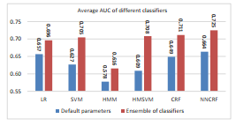Figure 1: Average AUC of different classifiers across all subjects. The blue bars correspond to the average AUC when the default value of the hyper-parameters have been used. The red bars correspond to the average AUC after using our ensemble learning algorithm. The numbers on top of each bar correspond to the AUC of each algorithm.

Qualitative comparison of different algorithms in Tables 1 suggests the following: 1) our proposed ensemble learning approach considerably improves the performance of any classifier for almost all subjects, 2) HMM is the worst performing classifier, 3) NNCRF outperforms other algorithms in terms of average AUC across all subjects on the test dataset, and 4) interestingly, for some subjects none of the discriminative sequence labeling classifiers had a good performance – this means that these classifiers are not able to capture the temporal structure of the signal in these subjects.

Table 1: The results of comparing different algorithms on the test dataset. Default is the results of using the default values of the hyper-parameters. Ensemble corresponds to the results of the ensemble learning approach. Highlighted cells show the algorithm for which the performance is the best.

LR

SVM

HMM

HSVM

CRF

NNCRF

Subject

Default

Ensemble

Default

Ensemble

Default              Ensemble

Default              Ensemble

Default

Ensemble

Default                  Ensemble

1 2 3 4 5 6 7 8 9 KT

0.617162 0.605175 0.66646 0.672782 0.559119 0.67886 0.725141 0.708607 0.616434 0.766713

0.708 ±0.003

0.471583 0.534574 0.659264 0.618411 0.559787 0.652671 0.710272 0.706152 0.606463 0.722982

0.684 ±0.008 0.668 ±0.002 0.721 ±0.004 0.758 ±0.003 0.622 ±0.007 0.729 ±0.003 0.778 ±0.002 0.736 ±0.002 0.638 ±0.007 0.818 ±0.002

0.4704 0.577131 0.64575 0.556342 0.510666 0.484071 0.605163 0.508587 0.527084 0.711457

0.572 ±0.003 0.647 ±0.014 0.688 ±0.003 0.571 ±0.004 0.509 ±0.003 0.63 ±0.015 0.71 ±0.01 0.633 ±0.034 0.598 ±0.013 0.732 ±0.006

0.566726 0.602029 0.642878 0.592601 0.509916 0.629371 0.68268 0.541939 0.564801 0.70759

0.682 ±0.004 0.647 ±0.003 0.724 ±0.001 0.749 ±0.004

0.554054 0.640085 0.689771 0.594204 0.473098 0.692138 0.671861 0.629435 0.591498 0.789081

0.651 ±0.006 0.66 ±0.004 0.735 ±0.002 0.725 ±0.006 0.618 ±0.006

0.565342

0.653 ±0.004 0.658 ±0.004

0.663 ±0.004 0.709 ±0.003

0.681072

0.691368 0.540245 0.493071 0.700657 0.666293 0.717994 0.588181 0.839713

0.743 ±0.004

0.769 ±0.002

0.722 ±0.003 0.632 ±0.004 0.73 ±0.006 0.755 ±0.004

0.629 ±0.003 0.692 ±0.004 0.762 ±0.002 0.729 ±0.002 0.626 ±0.006 0.826 ±0.004

0.655 ±0.003

0.718 ±0.002

0.731 ±0.005

0.802 ±0.002

0.751 ±0.003 0.697 ±0.011 0.669 ±0.005 0.871 ±0.005

0.658 ±0.013

0.779 ±0.004

0.687 ±0.009

0.686 ±0.003

0.827 ±0.004

0.881 ±0.004

CS CB ID

0.723935 0.610225 0.585436

0.733 ±0.004 0.597 ±0.002 0.605 ±0.002

0.727856 0.604169 0.573955

0.763 ±0.004 0.6 ±0.003 0.642 ±0.008

0.76225 0.547909 0.603535

0.637 ±0.01 0.554 ±0.006 0.518 ±0.004

0.706031 0.579983 0.588246

0.777 ±0.003 0.617 ±0.003 0.667 ±0.007

0.828081 0.615299 0.668705

0.831 ±0.004 0.626 ±0.005 0.682 ±0.011

0.797626

0.833 ±0.006

0.637969

0.631 ±0.003

0.706668

0.723±0.013

AVERAGE

0.657

0.696

0.627

0.705

0.578

0.616

0.609

0.708

0.649

0.711

0.664

0.725

To statistically compare the performance of the different classification methods, the Friedman statistical test was performed. The Friedman test [32] is a non-parametric statistical test, which ranks different classifiers for each subject separately. It then averages the ranks over all subjects. The algorithm with the lowest rank is the best performing one. Figure 2 shows the average rank of different classifiers. The best performing classifier is the ensemble of NNCRFs. In all classification algorithms, using the ensemble approach considerably improves the average rank.

In the Friedman test, the null hypothesis assumes that all algorithms have the same performance (thus, they have the same rank). After performing the Friedman test, the p-value was 4.34E-11. α was chosen to be 0.05. This p-value is low enough to reject the null hypothesis, therefore we conclude that the difference between algorithms is not random. Another set of statistical tests are performed to identify which algorithms are the source of difference. We conduct the Holm’s [32] test as the post-hoc statistical test. In the post-hoc test, we perform pairwise comparison of all the other classifiers versus the best classifier (i.e. ensemble of NNCRFs) in terms of the average rank.

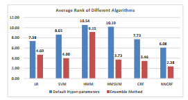Figure 2: Average rank of different classifiers across all subjects. The blue bars correspond to the average rank when the default value of the hyper-parameters have been used. The red bars correspond to the average rank after using our ensemble learning algorithm.

	Hypothesis	P-value
11	HMM vs. NNCRF(ensemble)	8.13E-09
10	HMSVM vs. NNCRF(ensemble)	3.37E-08
9	HMM(Ensemble) vs. NNCRF(ensemble)	1.70E-06
8	SVM vs. NNCRF(ensemble)	9.29E-06
7	CRF vs. NNCRF(ensemble)	1.57E-04
6	LR vs. NNCRF(ensemble)	4.07E-04
5	NNCRF vs. NNCRF(ensemble)	9.03E-03
4	LR(Ensemble) vs. NNCRF(ensemble)	1.03E-01
3	SVM(Ensemble) vs. NNCRF(ensemble)	2.53E-01
2	HMSVM(Ensemble) vs. NNCRF(ensemble)	3.41E-01
1	CRF(Ensemble) vs. NNCRF(ensemble)	4.46E-01

Table 2: P-values corresponding to pairwise comparison of different classifiers versus the best performing classifier. α is chosen to be 0.05. All hypothesis with p-value less than 0.001 are rejected.

In this statistical test, each null hypothesis states that the best classifier and the other classifier have the same mean rank. The p-values corresponding to pairwise comparison of classifiers are shown in Table-2. According to the Holms test results, the null hypothesis 1 through 5 are not rejected. This means that the difference between the ensemble of NNCRFs and other ensemble algorithms is not significant. However, the statistical tests show that the ensemble of NNCRFs is significantly better than nonensemble methods.

7          Conclusion

In this study, we proposed a discriminative sequence labeling algorithm (classifier), to capture the dynamics of the EEG signal. We evaluated the performance of our algorithm (which we denote as NNCRF) on two self-paced BCI datasets and showed that it is superior, compared to classical classifiers and sequence labeling classifiers. NNCRF is a combination of a neural network and a CRF classifier. We demonstrated that CRF and NNCRF can capture the temporal properties of the EEG signal and improve the accuracy of the BCI in most of the subjects. In some subjects however, the temporal structure of the EEG data is difficult to capture by these classifiers. The neural network part of NNCRF converts the original observation vector into a new representation which is then fed to the CRF part. The non-linear transformation (by the neural network) of the observation vector helps the CRF part to easily discriminate between the different control and NC.

Overall, the reason for the poor performance of classical approaches is that they do not exploit the dynamics of the EEG signal. As for the HMM, although this algorithm models the temporal correlations in an EEG signal, its poor performance stems from the fact that it focuses on learning each mental task separately (i.e. without learning to discriminate between them). On the other hand, discriminative sequence labeling classifiers do not only model the temporal properties of each mental task, they also model the transition from one metal task to another (e.g. transition from movement to NC state).

We also showed that using an ensemble of classifiers that have been trained on different parts of the BCI hyper-parameter space can further improve the performance. We used Bayesian optimization to find the different values of the BCI hyper-parameters. Selecting different values for the hyper-parameters exposes each individual classifier to different parts of the BCI hyper-parameter space. We believe that this diversification is the key to the superiority of using the ensemble of classifiers. The performance of each individual classifier is very sensitive to the choice of the hyper-parameters of the BCI and using an ensemble of classifiers can decrease the variance of the final classifier.

The best performing algorithm was the ensemble of NNCRF classifiers both in terms of the average rank and average AUC of the final classifier. We statistically compared the performance of different classifiers to the ensemble of NNCRFs. The results showed, for SVM, LR, HMSVM and CRF, the ensemble learning approach results in significantly better performance compared to the single classifier with default value of the hyper-parameters. For NNCRF, the Holm’s statistical test showed that the difference between NNCRF and the ensemble of NNCRF was not significant. However, the performance of the ensemble of NNCRFs was considerably better than the single NNCRF with default values of the hyperparameters.

In this study, we used linear chain discriminative sequence labeling classifiers, i.e. the type of the feature functions used in this study were all inspired by Hidden Markov Models. So they are all local in nature, with each feature function only depending on the current or the previous label in the sequence. It is possible to use global features such as the ones that capture higher orders of dependency of the transition between consecutive labels, or feature functions that capture dependency between the EEG signal and labels of the EEG signal from distant past. These types of feature functions have the ability to capture more complex structures in the data and increase the power of each individual classifier.

Appendix

1. Block Diagram of the Learning

Figure 3 shows a simple block diagram of one iteration of our ensemble learning algorithm (which is explained in Section 4). In our approach the BCI is like a self-regulating system which improves itself based on the feedback that it receives from the classification block. The cross-validation accuracy of the classifier is given to the Bayesian optimization block, and this block proposes new values for the hyperparameters for next iteration of the algorithm. The hyper-parameter values are used to extract features from the EEG signal, and a new classifier is trained using the features extracted from the training data. The extracted features are the power values in the frequency bands proposed by the Bayesian optimization block.

Each iteration of our ensemble learning approach generates a classifier (L_t). After running the algorithm for T iterations, we will have T different classifiers which are trained on different parts of the BCI hyper-parameter space. Eventually, the classifiers (L₁,L₂,…,L_T ) are combined (using averaging) to build a final classifier which is evaluated on the unseen test dataset.

Acknowledgments

This work was made possible by NPRP grant 7-6841-127 from the Qatar National Research Fund (a member of Qatar Foundation). The statements made herein are solely the responsibility of the authors.

1. J. R. Wolpaw, N. Birbaumer, D. J. McFarland, G. Pfurtscheller, T. M. Vaughan, Brain–computer interfaces for communication and control, Clinical neurophysiology 113 (6) (2002) 767–791.
2. A. Bashashati, R. K. Ward, G. E. Birch, Towards development of a 3-state self-paced brain-computer interface, Computational intelligence and neuroscience 2007.
3. J. F. D. Saa, M. etin, A latent discriminative model-based approach for classification of imaginary motor tasks from eeg data, Journal of Neural Engineering 9 (2) (2012) 026020.URL http://stacks.iop.org/1741-2552/9/i=2/a=026020
4. L. F. Nicolas-Alonso, R. Corralejo, J. Gomez-Pilar, D. lvarez, R. Hornero, Adaptive stacked generalization for multiclass motor imagery-based brain computer interfaces, IEEE Transactions on Neural Systems and Rehabilitation Engineering 23 (4) (2015) 702–712. doi:10.1109/TNSRE.2015.2398573.
5. Y. Song, F. Sepulveda, A novel onset detection technique for braincomputer interfaces using sound-production related cognitive tasks in simulated-online system, Journal of Neural Engineering 14 (1) (2017) 016019. URL http://stacks.iop.org/1741-2552/14/i=1/a=016019
6. Y. Yu, J. Jiang, Z. Zhou, E. Yin, Y. Liu, J. Wang, N. Zhang, D. Hu, A self-paced brain-computer interface speller by combining motor imagery and p300 potential, in: 2016 8th In-ternational Conference on Intelligent Human-Machine Sys-tems and Cybernetics (IHMSC), Vol. 02, 2016, pp. 160–163. doi:10.1109/IHMSC.2016.80.
7. T. G. Dietterich, Machine learning for sequential data: A review, in: Structural, syntactic, and statistical pattern recognition, Springer, 2002, pp. 15–30.
8. A. Bashashati, M. Fatourechi, R. K. Ward, G. E. Birch, A survey of signal processing algorithms in brain–computer interfaces based on electrical brain signals, Journal of Neural engineering 4 (2) (2007) R32.
9. C. S. L. Tsui, J. Q. Gan, S. J. Roberts, A self-paced brain– computer interface for controlling a robot simulator: an online event labelling paradigm and an extended kalman filter based algorithm for online training, Medical & biological engineering & computing 47 (3) (2009) 257–265.
10. M. Fatourechi, R. Ward, G. Birch, A self-paced brain– computer interface system with a low false positive rate, Journal of neural engineering 5 (1) (2007) 9.
11. G. Pfurtscheller, F. H. Lopes da Silva, Event-related eeg/meg synchronization and desynchronization: basic principles, Clinical neurophysiology 110 (11) (1999) 1842–1857.
12. L. R. Rabiner, A tutorial on hidden markov models and selected applications in speech recognition, Proceedings of the IEEE 77 (2) (1989) 257–286.
13. S. Chiappa, N. Donckers, S. Bengio, F. Vrins, Hmm and iohmm modeling of eeg rhythms for asynchronous bci systems, in: ESANN, 2004.
14. N. Nguyen, Y. Guo, Comparisons of sequence labeling algorithms and extensions, in: Proceedings of the 24th international conference on Machine learning, ACM, 2007, pp. 681–688.
15. D. L. Vail, M. M. Veloso, J. D. Lfferty, Conditional random fields for activity recognition, in: Proceedings of the 6th international joint conference on Autonomous agents and multiagent systems, ACM, 2007, p. 235.
16. H. Bashashati, R. K. Ward, A. Bashashati, Hidden markov support vector machines for self-paced brain computer interfaces, in: 2015 IEEE 14th International Conference on Machine Learning and Applications (ICMLA), 2015, pp. 382–385. doi:10.1109/ICMLA.2015.178.
17. B. A. S. Hasan, J. Q. Gan, Conditional random fields as classifiers for three-class motor-imagery braincomputer interfaces, Journal of Neural Engineering 8 (2) (2011) 025013.URL http://stacks.iop.org/1741-2552/8/i=2/a=025013
18. D. Saa, F. Jaime, M. Cetin, Discriminative methods for classification of asynchronous imaginary motor tasks from eeg data, Neural Systems and Rehabilitation Engineering, IEEE Trans-actions on 21 (5) (2013) 716–724.
19. J. Lafferty, A. McCallum, F. Pereira, Conditional random fields: Probabilistic models for segmenting and labeling sequence data, in: Proceedings of the eighteenth international conference on machine learning, ICML, Vol. 1, pp. 282–289.
20. I. Tsochantaridis, T. Hofmann, T. Joachims, Y. Altun, Support vector machine learning for interdependent and structured output spaces, in: Proceedings of the twenty-first international conference on Machine learning, ACM, 2004, p. 104.
21. C.-W. Hsu, C.-C. Chang, C.-J. Lin, et al., A practical guide to support vector classification.
22. C. M. Bishop, Pattern recognition and machine learning, Vol. 1, springer New York, 2006.
23. J. Snoek, H. Larochelle, R. P. Adams, Practical bayesian optimization of machine learning algorithms, in: Advances in Neural Information Processing Systems, 2012, pp. 2951–2959.
24. M. Tangermann, K.-R. Mller, A. Aertsen, N. Birbaumer, C. Braun, C. Brunner, R. Leeb, C. Mehring, K. Miller, G. Mueller-Putz, G. Nolte, G. Pfurtscheller, H. Preissl, G. Schalk, A. Schlgl, C. Vidaurre, S. Waldert, B. Blankertz, Review of the bci competition iv, Frontiers in Neuroscience 6 (2012) 55. doi:10.3389/fnins.2012.00055. URL http://journal.frontiersin.org/article/10.3389/ fnins.2012.00055
25. J. F. Borisoff, S. G. Mason, A. Bashashati, G. E. Birch, Brain-computer interface design for asynchronous control applications: improvements to the lf-asd asynchronous brain switch, Biomedical Engineering, IEEE Transactions on 51 (6) (2004) 985–992.
26. T. Do, T. Arti, et al., Neural conditional random fields, in: International Conference on Artificial Intelligence and Statistics, 2010, pp. 177–184.
27. J. Peng, L. Bo, J. Xu, Conditional neural fields, in: Advances in neural information processing systems, 2009, pp. 1419–1427.
28. H. Bashashati, R. K. Ward, A. Bashashati, User-customized brain computer interfaces using bayesian optimization, Journal of Neural Engineering 13 (2) (2016) 026001. URL http://stacks.iop.org/1741-2552/13/i=2/a=026001
29. E. Brochu, V. M. Cora, N. De Freitas, A tutorial on bayesian optimization of expensive cost functions, with application to active user modeling and hierarchical reinforcement learning, arXiv preprint arXiv:1012.2599.
30. H. Ramoser, J. Muller-Gerking, G. Pfurtscheller, Optimal spatial filtering of single trial eeg during imagined hand movement, Rehabilitation Engineering, IEEE Transactions on 8 (4) (2000) 441–446.
31. Y. Altun, I. Tsochantaridis, T. Hofmann, et al., Hidden markov support vector machines, in: ICML, Vol. 3, 2003, pp. 3–10.
32. J. Demsar, Statistical comparisons of classifiers over multiple data sets, The Journal of Machine Learning Research 7 (2006) 1–30.

(Click to view)

(Click to view)