Analysis of Wireless Traffic Data through Machine Learning
Analysis of Wireless Traffic Data through Machine Learning
Volume 2, Issue 3, Page No 865-871, 2017
Author’s Name: Muhammad Ahsan Latif1, a), Muhammad Adnan2
View Affiliations
1Department of Computer Science, University of Agriculture Faisalabad, 38000, Pakistan
2Research assistant, Institute of Manufacturing Information and Systems, Department of Computer Science, National Cheng Kung University(NCKU), 701, Tainan, Taiwan
a)Author to whom correspondence should be addressed. E-mail: mahsanlatif@uaf.edu.pk
Adv. Sci. Technol. Eng. Syst. J. 2(3), 865-871 (2017); ![]() DOI: 10.25046/aj0203107
DOI: 10.25046/aj0203107
Keywords: NextGen wireless networks, Resource management, Neural networks, Principal component analysis

Export Citations
The paper presents an analytical study on a wireless traffic dataset carried out under the different approaches of machine learning including the backpropagation feedforward neural network, the time-series NARX network, the self-organizing map and the principal component analyses. These approaches are well-known for their usefulness in the modeling and in transforming a high dimensional data into a more convenient form to make the understanding and the analysis of the trends, the patterns within the data easy. We witness to an exponential rise in the volume of the wireless traffic data in the recent decade and it is increasingly becoming a problem for the service providers to ensure the QoS for the end-users given the limited resources as the demand for a larger bandwidth almost always exist. The inception of the next generation wireless networks (3G/4G) somehow provide such services to meet the amplified capacity, higher data rates, seamless mobile connectivity as well as the dynamic ability of reconfiguration and the self-organization. Nevertheless, having an intelligent base-station able to perceive the demand well before the actual need may assist in the management of the traffic data. The outcome of the analysis conducted in this paper may be considered in designing an efficient and an intelligent base-station for better resource management for wireless network traffic.
Received: 23 April 2017, Accepted: 02 June 2017, Published Online: 20 June 2017
1. Introduction
Today, the communication has become an integral part of the daily activities for everyone. For example, the services such as video on demand (VoD), downloading music, stream video data, voice over IP (VoIP) and live video conference calls have become a part of the daily activities of the users. Such applications need a high quality of service, particularly for voice in real time. Resultantly, a lot of wireless technologies such as 3rd Generation (3G), wireless fidelity (Wi-Fi), Worldwide Interoperability Microwave Access (WiMAX), Global System for Mmobile Communications (UMTS) and the Evolution of the Long-Term (LTE) are growing to meet the accelerated needs of the users to provide them anywhere, anytime access to the Internet. In the recent past, the main point in the telecommunications sector is the next generation wireless networks (NGWNs). These networks consist of different techniques to gain access to the network to provide unlimited access to the internet, global roaming, high-speed and an increased user satisfaction.
The NextGen Wireless Networks are a combination of circuit-switched networks, various services, and packet switching. It is covering a wider area in which the user can take advantage of different wireless networks to improve the call quality. NextGen comprises of the services independent of the core technologies related to transport [1, 2]. It can be defined as a complex process, easily accessible, convenient and converging economic, efficient and flexible, personal and real, reliable and secure [3].
The fundamental technical issues for the NextGen Wireless Networks include end-to-end QoS, mobility management, energy efficiency, call admission control, resource allocation, and security. This has encouraged many researchers to develop the QoS models for the NextGen Wireless Networks [4]. In mobility the connected base station cannot support the ongoing session, and it has to handover the session to the new base station [5]. Under the wireless communication, most of the network equipment operate on battery power and with the limited resources just not capable to provide the energy to keep the equipment alive for extended time period [6]. Controlling calls in wireless communication is a process of administering the traffic volume. The decision of whether a new call has to be admitted, delayed, dropped or forwarded to a neighboring network is decided by this sub-system. The incoming traffic can further be split into real time i.e. video and voice, and non-real time i.e. images, text, etc. [7]. As the NextGen Wireless Networks are distributed and open architectures so it offers easy access to the services, information and the resources together with constant abuse from the fraudsters, hackers and crime units [8]. User identification based on the IP layer can be easily tampered within such networks. The packets sent over the network can be easily identified with a “borrowed” IP address, which grants the unauthorized users to mimic the valid ones. These intruders abuse services and gets benefit with the expenditures of legitimate users, who do not know the actual situation [9]. Such intruders can get a valid electronic serial number and mobile identification number during the registration process of the call. They can duplicate the same number on the other handset and utilize the services in the name of real user. A mobile node utilizes Mobile IP and Session Initiation Protocol (SIP) under subscriber mobility [10]. The installation of small cell base stations on the existing macro cellular systems is presented as a solution for an optimized coverage, offloading traffic and to boost the capacity of the next generation wireless networks in [11]. A comprehensive overview of the machine learning approaches used to address different issues in the wireless sensor network is provided in [12]. The researchers supported the use of machine learning techniques to better monitor the dynamic behavior that emerges out of the sensor network over time. For enhanced traffic management, the researchers performed classification of the traffic data through supervised machine learning approaches [13]. For mobile big data, the challenges of computing capabilities, spectrum efficiency and backhaul / fronthaul link capacity are discussed in [14]. The study presented different opportunities and the bottlenecks in the design of the scalable wireless systems to get adapt to the big data.
The foremost issue in the NextGen Wireless Networks is guaranteeing the QoS and provision of requisite resources to the connected subscribers from the service provider at any time. This claims the network reliability, bandwidth, timeliness, jitter, fault tolerance and seamless mobility among heterogeneous access networks. These needs are the driving factors for the NextGen Wireless Networks. Particularly, VoIP will be the most popular application in the future. It demands high QoS for the moving user. In this regard, many problems exist to make the NextGen Wireless Networks fully resourceful and well-matched with the existing services and technologies. For the moving subscribers providing the required service, by sustaining the adequate QoS while considering the various networks as well as the global roaming is a tricky job. The appearance of the irregular needs in the NextGen Wireless Networks require an effective assurance to satisfy the subscribers.
To ensure the QoS for the subscribers, an understanding of the behavior of the network traffic is necessary. This would assist in following an adaptive policy for using the available network resources to guarantee QoS at an optimal level. To analyze the network traffic behavior, we used the self-organizing map and further employed the principal component analyses. An intelligent module within a base-station could be embedded with the outcomes of the analysis to take adaptive decisions intelligently. The module would estimate the future requirements of the bandwidth for a base-station as per the previous history and commit in advance the requisite resources from the backhaul network for the guaranteed bandwidth provision to the end-users. The real time data of a 3G wireless network established by the Pakistan Telecommunication Co. LTD i.e. CDMA2000 1xEV-DO Rev is used in this study.
2. Intelligent Base Station
A schematic diagram of an intelligent base station is shown in Figure 1.
Following are the components of this intelligent model:
- Monitoring Unit: This component monitors the data transferred from the Base Station to the connected subscribers periodically.
- Storage Unit: This component stores the observed data in the memory to use for another component of this model i.e. Intelligent Forecasting Unit.
Intelligent Forecasting Unit: This component is the heart of the model, which facilities in forecasting of upcoming demands on the Base Station in a specific hour. It uses the previous stored data from the storage unit for predicting the upcoming resources requirement and subsequently forwards the request to the backhaul network in advance to allocate the forecasted bandwidth allocation.
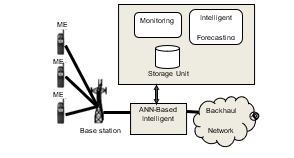
Figure 1: Intelligent base station model
3. Neural Network Based Analysis
The ANNs, owning a proven learning paradigm can be used effectively to develop such intelligent agent [15-27]. Three different NNs are tested to understand the patterns and the behavior lying within the network traffic data. The backpropagation feedforward neural network and the nonlinear autoregressive with external input neural network are used to better learn the demand time-wise. Whereas the self-organizing map is used to learn the key parameters to focus on. The training data comprises of the six-month wireless traffic data acquired from the Pakistan Telecommunication Company Ltd. The training data comes in periodic shape i.e. hourly data with reference to the week-days and an average accumulative throughput in a particular hour. The mathematical models of the three NNs are given as under.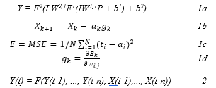
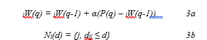
The (1) define the feedforward neural network completely. The (1a) defines a three layered architecture with LW as the layer weights, IW as the input weight matrices and P as the input vector The sub-equation (1b) gives the learning rule to update the network parameters wherein Xk represents the vector of the current weights and the biases, gk is the current gradient and ak is the learning rate. The (1c) defines the mean square error (mse) which is also one of the stopping criteria used during the training phase. The (1d) defines the relation how to determine the gradient. The system of nonlinear autoregressive with external input (NARX) is defined in (2). In our case, the previous two terms (of both the input & output) are taken into account to calculate the current term. The model uses the same learning rule as given in (1b). The system of (3) provides the rule to update the weights of the winning neuron as well as of the neighboring neurons in a neighborhood d’ defined in (3b). All of the three models are programmed and tested in Matlab. The used parameters are given in the following tables Table-1, Table-2 and Table-3 against each model.
The results of all the three models provide a very clear understanding of the relations among the variables embedded in the data. The function approximation performed by the feedforward model (1) provides a strong evidence of the relation between the output variable (throughput) and the input-vector (comprising of eight input elements). The training-performance for the feedforward model went perfectly well as shown in Figure-2 as all the three segments of the training data sets, i.e., the training, the testing and the validation got to converge optimally. The value of ‘R’ achieved in this case is R = 0.9867 (regression value).
The NARX model (2) is also found capable of learning the underlying behavior of the network traffic data. The function Bayesian Regularization is used for training purpose as it produces the better generalization for a complex and noisy data. The principle of adaptive weight minimization is followed to stop the training. In this model, the previous two states of the input-time-series and the target-time-series are taken into account to predict the next value in the output-time-series. The regression value is found to an acceptable level as R=0.983. An important graph of the NARX model, i.e., the time-series response is shown in Figure-3. A close similarity can be seen between the outputs and the targets. The lower part of the graph shows the error graph which is found well within the confidence interval. The objective of testing the SOM model over the traffic data is to reduce the data-dimensionality to see which variables are more intrinsic to the resource-requirement. A network of 100 neurons fully mapped the underlying data space. The impact of the variables on the network is fully conveyed in the input weight-planes. All the input weight-planes corresponding to the input variables are given in the Figure-4. The weight-planes for the input-1 to the input-7 contain most of the part as dark regions indicating zero or lower values for the weights between the network-neurons and that particular input. This would suggest the days of the week are not to play much role in deciding the network resource management as the traffic varies. The weight-plane for the 8th input variable, i.e., the hours, comprised of more bright spots and fewer dark ones presenting a strong connection strength with the network-neurons. The 9th weight-plane owns much of the bright spots as compared to the rest of the weight-planes showing the resilient connections with the neurons of the network.
|
(Dataset Distribution-%) Training/Testing/Validation |
(70)(15)15) |
| ANN Architecture | 8-25-1 |
| No. of input neuron | 8 |
| No. of hidden layer | 1 |
| No. of output neuron | 1 |
| Training Algorithm | Levenberg-Marquardt |
| Error performance function | MSE |
| Maximum Epochs | 1000 |
Table. 1. Parameters used for Feedforward ANN Model
|
(Dataset Distribution-%) Training/Testing/Validation |
(70)(15)15) |
| ANN Architecture | A 3-layered time delay network |
| No. of input neuron | 8 |
| No. of hidden layer | 1 |
| No. of output neuron | 1 |
| Training Algorithm | Bayesian Regulation |
| Error performance function | MSE |
| Maximum Epochs | 1000 |
Table. 2. Parameters used for NARX Model
| SOM Architecture | 10 x 10 |
| Neighborhood size | 3 x 3 |
| No. of input neurons | 9 |
| No. of output neurons | 100 |
| Training Algorithm | Batch weight / Bias |
| Error performance function | MSE |
| Maximum Epochs | 200 |
Table. 3. Parameters used for SOM Model
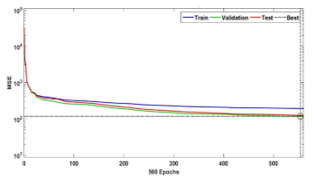
Figure 2. Feedforward Training Performance
1. Principal Component Analysis
The principal component analysis is regarded as one of the fundamental approach to simplify the data. A wide use of this approach has been reported in the relevant literature [28-29-30]. The approach basically transforms a redundant data comprising of linearly correlated variables into a non-redundant dataset of orthogonal (uncorrelated) variables. The transformation results into a projection of the existing data to a new data-space where each axis corresponds to an orthogonal variable, i.e., principal component. The principal components are arranged in terms of their variance, i.e., the first component (axis) holds the maximum variance, the second component, being orthogonal to the first component, holds the second-highest variance along its axis and so on. This projection highlights the real trends within the data which drive the overall behavior of the data. In the following, the results of the approach are presented conducted on wireless traffic dataset. The dataset is comprised of nine variables.
| Principal Components | Latent | Explained (%) |
| 1 | 1.60 | 17.85 |
| 2 | 1.16 | 12.96 |
| 3 | 1.16 | 12.96 |
| 4 | 1.16 | 12.96 |
| 5 | 1.16 | 12.96 |
| 6 | 1.16 | 12.96 |
| 7 | 1.14 | 12.73 |
| 8 | 0.41 | 4.590 |
| 9 | 1.53e-28 | 1.70e-27 |
Table 4. Variances of Principal Components
4. Principal Component Analysis
The principal component analysis is regarded as one of the fundamental approach to simplify the data. A wide use of this approach has been reported in the relevant literature [28-29-30]. The approach basically transforms a redundant data comprising of linearly correlated variables into a non-redundant dataset of orthogonal (uncorrelated) variables. The transformation results into a projection of the existing data to a new data-space where each axis corresponds to an orthogonal variable, i.e., principal component. The principal components are arranged in terms of their variance, i.e., the first component (axis) holds the maximum variance, the second component, being orthogonal to the first component, holds the second-highest variance along its axis and so on. This projection highlights the real trends within the data which drive the overall behavior of the data. In the following, the results of the approach are presented conducted on wireless traffic dataset. The dataset is comprised of nine variables.
| Principal Components | Latent | Explained (%) |
| 1 | 1.60 | 17.85 |
| 2 | 1.16 | 12.96 |
| 3 | 1.16 | 12.96 |
| 4 | 1.16 | 12.96 |
| 5 | 1.16 | 12.96 |
| 6 | 1.16 | 12.96 |
| 7 | 1.14 | 12.73 |
| 8 | 0.41 | 4.590 |
| 9 | 1.53e-28 | 1.70e-27 |
The variance and the variance-percentage for each principal component is given in the Table 4. This shows only the very first principal component contributes more in terms of variance as its share is 17.85 %. Most of the principal components, i.e., from 2 to 7 have almost a constant share of variance whereas the last two components present negligible share. Figure-5 provides a graphical representation of the share of each principal component variance-wise. In general cases, the first three or four principal components are considered enough to represent much of the variance in the data but in our case except the very last two principal components, all of the first seven principal components contribute significantly in the variance. In Figure-6 all the nine variables are represented as vectors wherein the direction and the length of each vector shows the contribution of each vector to the first two principal axis. For example, the first principal component along the horizontal axis, has the positive coefficients for the variables Hr. (hour), Throughput, Sunday, Saturday, Friday and Thursday. This gives an idea that more variance occur in these days. The maximum variance are for the variables Hr. and the Throughput as both are also in complete parallel to the component’ axis. This also shows that the variables Mon, Wed and Tue have no influence on the first principal component as these fall on the negative side of the horizontal axis. The second principal component, on the vertical axis, has positive coefficients for the variables Mon, Wed, Sun, Sat, Hr. and Throughput whereas the negative coefficient for Tue, Fri and Thu. The PCA analysis shows the main driving forces behind the variances in the data come from the variable Hr., Throughput and the days like Thu, Fri, Sat and Sun. These results are in complete compliance with the findings of self-organization map presented in Figure-4. The weights of the network out of the input-9 (Throughput) and the input-8 (Hr.) are much stronger as compared to the weights from the remaining inputs. Also the weights from the input-4, input-5, input-6 and input-7 (correspond to Thu, Fri, Sat and Sun) contain slightly more grey areas as compared to the weights from the remaining counterparts, i.e., input-1, input-2 and input-3 which correspond to Mon, Tue and Wed.
5. Results and Discussion
The results of all the three models provide a very clear understanding of the relations among the variables embedded in the data. The function approximation performed by the feedforward model (eq. 1) provides a strong evidence of the relation between the output variable (throughput) and the input-vector (comprising of eight input elements). The training-performance for the feedforward model went perfectly well as shown in Figure-2 as all the three segments of the training data sets, i.e., the training, the testing and the validation got to converge optimally. The value of ‘R’ achieved in this case is R The NARX model (eq. 2) is also found capable of learning the underlying behavior of the network traffic data. The function Bayesian Regularizationis used for training purpose as it produces the better generalization for a complex and noisy data. The principle of adaptive weight minimization is followed to stop the training. In this model, the previous two states of the input-time-series and the target-time-series are taken into account to predict the next value in the output-time-series. The regression value is found to an acceptable level as R=0.983. An important graph of the NARX model, i.e., the time-series response is shown in Figure-3. A close similarity can be seen between the outputs and the targets. The lower part of the graph shows the error graph which is found well within the confidence interval. The objective of testing the SOM model over the traffic data is to reduce the data-dimensionality to see which variables are more intrinsic to the resource-requirement. A network of 100 neurons fully mapped the underlying data space. The impact of the variables on the network is fully conveyed the input weight-planes. All the input weight-planes corresponding to the input variables are given in the Figure-4. The weight-planes for the input-1 to the input-7 contain most of the part as dark regions indicating zero or lower values for the weights between the network-neurons and that particular input. This would suggest the days of the week are not to play much role in deciding the network resource management as the traffic varies. The weight-plane for the 8th input variable, i.e., the hours, comprised of more bright spots and fewer dark ones presenting a strong connection strength with the network-neurons. The 9th weight-plane owns much of the bright spots as compared to the rest of the weight-planes showing the resilient connections with the neurons of the network. The results from PCA analysis confirm the neural-network based modeling. The analysis presented here as a case study for the network traffic data shows a strong potential to employ the machine learning techniques to manage the network traffic. With the surging rate of network traffic across different platforms and networks, the provision of QoS has become an issue for the service providers especially for the telecom industry. The communication has taken multi-dimensional shape, i.e., voice, video, text, etc., all being delivered over the same infrastructure. Though, new paradigms for the increased band-width, improved communication protocols, etc., are being worked on in parallel yet the efforts should also be made to better plan the network traffic within the same framework to ensure the maximum optimum use of the existing resources. In this regard, the machine learning approaches may play a significant role to assist the service providers in dealing with the traffic management. More research is required in this context to develop robust traffic planning.
6. Conclusion
The behavior of the wireless traffic data is studied under neural networks and the principal component analysis. The three ANN models used include backpropagation feedforward, the time-series NARX and the self-organizing map. The FF model and the NARX model showed the potential to closely model the relation between the throughput and the other variables. The results from the SOM model showed the dimension reduction in the original data by presenting strong weight diagrams for only the two inputs while representing the remaining inputs with average weight strengths. The results from the principal component analysis further verify the results from the SOM. The results of all this study could be incorporated in designing an intelligent module at a network base station to provide adaptive services for the better resource management, hence improving the efficiency of the network.
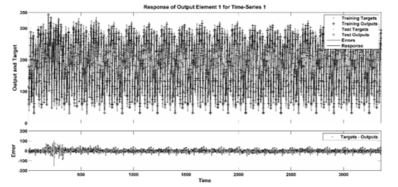
Figure. 3. Time series response of NARX model
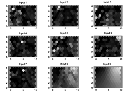
Figure. 4. Some weight planes for the inputs
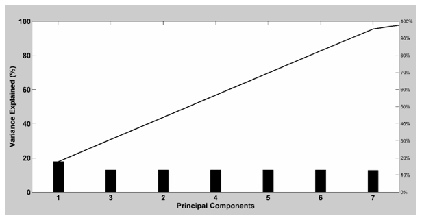
Figure. 5 Variance-Percentage of principal components
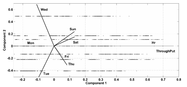
Figure. 6 Projection of all the variables onto the first two orthogonal principal components
- Latif, M. Ahsan, and M. Adnan. “ANN-Based Data Mining for Better Resource Management in the Next Generation Wireless Networks.” Frontiers of Information Technology (FIT), 2016 International Conference on. IEEE, 2016.
- Lee, Chae-Sub, and N. Morita. “Next Generation Network Standards in ITU-T.” 2006 1st IEEE International Workshop on Broadband Convergence Networks.
- Korotky, Steven K., and Thomas Pfeiffer. “Continuing advances in next-generation communication technologies, services, and networks.” Bell Labs Technical Journal 14.1 (2009): 1-5.
- Li, Bo, et al. “QoS enabled voice support in the next generation Internet: issues, existing approaches and challenges.” IEEE Communications Magazine 38.4 (2000): 54-61.
- Akyildiz, Ian F., Jiang Xie, and Shantidev Mohanty. “A survey of mobility management in next-generation all-IP-based wireless systems.” IEEE Wireless communications 11.4 (2004): 16-28.
- Berardi, Victor L., and Guoqiang Peter Zhang. “An empirical investigation of bias and variance in time series forecasting: modeling considerations and error evaluation.” IEEE Transactions on Neural Networks 14.3 (2003): 668-679.
- Wu, Chen-Feng, et al. “A novel call admission control policy using mobility prediction and throttle mechanism for supporting QoS in wireless cellular networks.” Journal of Control Science and Engineering 2011 (2011): 21.
- Bella, MA Bihina, M. S. Olivier, and J. H. P. Eloff. “A fraud detection model for Next-Generation Networks.” Proceedings of the 8th Southern African Telecommunications Networks and Applications Conference (SATNAC 2005), Central Drakensberg, KwaZulu-Natal, South Africa. 2005.
- Ericsson 2004. Categorizing telecommunications fraud, an introduction for those new to the subject.
- Lee, Hyejeong, Sung Won Lee, and Dong-Ho Cho. “Mobility management based on the integration of mobile IP and session initiation protocol in next generation mobile data networks.” Vehicular Technology Conference, 2003. VTC 2003-Fall. 2003 IEEE 58th. Vol. 3. IEEE, 2003.
- Bennis, Mehdi, et al. “When cellular meets WiFi in wireless small cell networks.” IEEE Communications Magazine 51.6 (2013): 44-50.
- Alsheikh, Mohammad Abu, et al. “Machine learning in wireless sensor networks: Algorithms, strategies, and applications.” IEEE Communications Surveys & Tutorials 16.4 (2014): 1996-2018.
- Ertam, Fatih, and Engin Avci. “Classification with intelligent systems for internet traffic in enterprise networks.” Int. J. Comput. Commun. Instrum. Eng 3 (2013): 1469-2349.
- Bi, Suzhi, et al. “Wireless communications in the era of big data.” IEEE Communications Magazine 53.10 (2015): 190-199.
- Atiya, Amir F., et al. “A comparison between neural-network forecasting techniques-case study: river flow forecasting.” IEEE Transactions on neural networks 10.2 (1999): 402-409.
- Balkin, Sandy D., and J. Keith Ord. “Automatic neural network modeling for univariate time series.” International Journal of Forecasting 16.4 (2000): 509-515.
- Chen, Yuehui, et al. “Time-series forecasting using flexible neural tree model.” Information sciences 174.3 (2005): 219-235.
- Cottrell, Marie, et al. “Neural modeling for time series: a statistical stepwise method for weight elimination.” IEEE Transactions on Neural Networks 6.6 (1995): 1355-1364.
- Giordano, Francesco, Michele La Rocca, and Cira Perna. “Forecasting nonlinear time series with neural network sieve bootstrap.” Computational Statistics & Data Analysis 51.8 (2007): 3871-3884.
- Günther, Frauke, and Stefan Fritsch. “neuralnet: Training of neural networks.” The R journal 2.1 (2010): 30-38.
- Jain, Ashu, and Avadhnam Madhav Kumar. “Hybrid neural network models for hydrologic time series forecasting.” Applied Soft Computing 7.2 (2007): 585-592.
- Kaastra, Iebeling, and Milton Boyd. “Designing a neural network for forecasting financial and economic time series.” Neurocomputing 10.3 (1996): 215-236.
- Lapedes, Alan, and Robert Farber. Nonlinear signal processing using neural networks: Prediction and system modelling. No. LA-UR-87-2662; CONF-8706130-4. 1987.
- Zhang, Guoqiang, B. Eddy Patuwo, and Michael Y. Hu. “Forecasting with artificial neural networks:: The state of the art.” International journal of forecasting 14.1 (1998): 35-62.
- Poli, I., and R. D. Jones. “A neural net model for prediction.” Journal of the American Statistical Association 89.425 (1994): 117-121.
- Weigend, Andreas S., Bernardo A. Huberman, and David E. Rumelhart. “Predicting the future: A connectionist approach.” International journal of neural systems 1.03 (1990): 193-209.
- Zhang, Guoqiang, B. Eddy Patuwo, and Michael Y. Hu. “Forecasting with artificial neural networks:: The state of the art.” International journal of forecasting 14.1 (1998): 35-62.
- Le Borgne, Yann-Aël, Sylvain Raybaud, and Gianluca Bontempi. “Distributed principal component analysis for wireless sensor networks.” Sensors 8.8 (2008): 4821-4850.
- Le Borgne, Y., and Gianluca Bontempi. “Unsupervised and supervised compression with principal component analysis in wireless sensor networks.” Proceedings of the Workshop on Knowledge Discovery from Data, 13th ACM International Conference on Knowledge Discovery and Data Mining. 2007.
- Li, J., and Y. Zhang. “Interactive sensor network data retrieval and management using principal components analysis transform.” Smart Materials and Structures 15.6 (2006): 1747.