A novel model for Time-Series Data Clustering Based on piecewise SVD and BIRCH for Stock Data Analysis on Hadoop Platform
A novel model for Time-Series Data Clustering Based on piecewise SVD and BIRCH for Stock Data Analysis on Hadoop Platform
Volume 2, Issue 3, Page No 855-864, 2017
Author’s Name: Ibgtc Bowala1, Mgnas Fernando2, a)
View Affiliations
1Undergraduate, University of Colombo school of Computing, 00700, Sri Lanka
2Senior Lecturer, University of Colombo school of Computing, 00700, Sri Lanka
a)Author to whom correspondence should be addressed. E-mail: nas@ucsc.cmb.ac.lk
Adv. Sci. Technol. Eng. Syst. J. 2(3), 855-864 (2017); ![]() DOI: 10.25046/aj0203106
DOI: 10.25046/aj0203106
Keywords: Clustering, Time series analysis, SVD, BIRCH, Hadoop, MapReduce

Export Citations
With the rapid growth of financial markets, analyzers are paying more attention on predictions. Stock data are time series data, with huge amounts. Feasible solution for handling the increasing amount of data is to use a cluster for parallel processing, and Hadoop parallel computing platform is a typical representative. There are various statistical models for forecasting time series data, but accurate clusters are a pre-requirement. Clustering analysis for time series data is one of the main methods for mining time series data for many other analysis processes. However, general clustering algorithms cannot perform clustering for time series data because series data has a special structure and a high dimensionality has highly co-related values due to high noise level. A novel model for time series clustering is presented using BIRCH, based on piecewise SVD, leading to a novel dimension reduction approach. Highly co-related features are handled using SVD with a novel approach for dimensionality reduction in order to keep co-related behavior optimal and then use BIRCH for clustering. The algorithm is a novel model that can handle massive time series data. Finally, this new model is successfully applied to real stock time series data of Yahoo finance with satisfactory results.
Received: 21 April 2017, Accepted: 31 May 2017, Published Online: 20 June 2017
1. Introduction
A stock market, equity market or share market is the aggregation of buyers and sellers of stocks, which enables the trading of company stocks collective shares [1]. With the rapid development of trades in the world, people are paying more attention on investing in Stock markets [1]. By reviewing the stock’s financial curves, an educated decision can make whether the company is stable, growing and has an improving future. Thus, it is necessary to find a way to identify stocks with similar trend curves, which is very difficult due to uncertainty [2]. Financial institutes such as stock markets produce massive datasets [1]. Large amount of data is a barrier to analyze and summarize stock market data.
To visualize stock market behavior, researchers have used data mining techniques such as decision tree [1,3], neural network [1,4], association rules [5], factor analysis [6], etc. The decision trees are a powerful beginning step, but very costly. Neural networks (NN) such as Self-Organizing Feature Maps (SOFM) have been effectively applied in a many previous approaches. However, using decision trees or NNs for cluster large data sets cause performance degradation. Association rule is a popular and well-studied method for discovering interesting relations among variables in huge databases. But, researchers have also shown that it can produce better index return only with fewer trades. Factor analysis is an important step towards effectual clustering. But it can use only a limited number of stocks and, can only find fewer relations like the best stock. The overall analysis for large number of stocks cannot be achieved using factor analysis.
Clustering, which is another tool for data analysis [3,13], provides the basis for most of the data analysis, decision making, designing, and forecasting problems. Thus, it is very important to achieve accurate clusters. But, due to the special structure of time-series data with high level of noise, building an effective model for clustering needs a huge effort and time. Furthermore, building an effective model for time series clustering cannot be achieved without a comprehensive study of theories and previous approaches.In statistics, signal processing and many other fields, a time series is a sequence of data points measured typically at successive [7] uniform times [1]. Stock data, being time series data, shares a common set of analysis problems with other time-series data. Time-series analysis includes methods that attempt to understand time series, to make forecasts [1]. Time-series data are often large and might contain outliers. In addition, time series are a special type of data set where elements have a temporal order [8] and time-series data are essentially high-dimensional data [7]. Mining high-dimensional data involves handling a range of challenges such as curse of dimensionality, the meaningfulness of the similarity measure in the high-dimensional space, and handling outliers. Furthermore, time series analysis requires multiple arrays to represent the series, which make it computationally very expensive. Therefore, an effective dimensionality-reduction method is needed to reduce memory consumption and to fit matrix into memory and it should capture the temporal order and the highly-correlated features of time series [7]. Today, dimension reduction [7,8,9] is a highly-attractive research area and researchers focus on new techniques for dimension reduction [10,11,12] because it affects both the accuracy and the efficiency. The stock data only differs from other time-series data in terms of the data distribution. Therefore, our primary focus of research is time-series analysis.
Moreover, due to the volatility of stock data, which is not directly recognizable [2,14], and due to the type of distribution of stock data, the clustering becomes harder. Unlike financial return series, price series is harder to handle, because it has more attractive statistical properties [2]. Even for a stock return series, the volatility is not directly recognizable and it becomes harder as far as the price curves are concerned. Thus, the financial analysis sector has a thirsty of identifying relationships between original price curves, rather than trend and other curves.
Many stock analysis researchers and companies are searching for the right methods to cluster stock data in order to perform their analysis. This paper introduces a novel model for time-series clustering, including a new dimensionality-reduction approach. This can be taken as a case study for time-series clustering big-data fields. Comparative decisions made in the noise removal stage enhanced the clustering quality. The novel dimensionality-reduction approach is suitable for time-series data, for stock data, and for other huge data sets. The novel model is applied successfully on real stock data of Yahoo finance to evaluate the accuracy and performances. The cluster evaluation shows that, this can cluster stock price curves very effectively and efficiently. The next section will discuss the related work.
2. Related Work
A time series is “a sequence of observed data over time”, where are time units and is the number of observations [7]. It has a temporal order [8], often large and might contain outliers and essentially high-dimensional data [7]. The time series X can be considered as a point in n-dimensional space. This suggests that time series could be clustered using clustering methods. Time series tend to contain highly-correlated features. Thus, time-series data are usually good applicants for dimensionality reduction [9].
Let be the price of an asset at time index . Thus, the One-Period Simple Return is holding the asset for one period from date to date would result in a simple gross return of [2]. Stock return series data follows a normal distribution of [14], where mean and is the variance.
In order to reduce defects in the clustering stage, data standardizing is needed [13]. Calculating the mean absolute deviation and calculating the standardized measurement (z-score) are some methods. Z-score is defined as , where is the mean and is the standard deviation of the sequence.
Some of the dimensionality reduction techniques researchers which have been using for time-series data are Singular Value Decomposition (SVD) [7,9,14,15], the Discrete Fourier transforms (DFT) [7,9,16], the Discrete Wavelets Transform (DWT) [7,9,17], Piecewise Aggregate Approximation (PAA) [7,9], Principal component analysis (PCA) [12,18], Factor analysis (FA) [12,19], Adaptive Piecewise Constant Approximation (APCA) [7], Piecewise Linear Approximation (PLA) [7], Independent component analysis (ICA), Chebyshev Polynomials (CHEB) [7], etc. Researchers have been using wavelets for dimension reduction [7,9,17] but, its only defined for sequences with length which are an integral power of two [9]. Therefore, this method cannot be used for time series processing with various lengths, which is a very huge limitation. PAA ignores the co-related behavior of time-series data. Thus, PAA is not a good solution to use for dimension reduction of time-series data.
Singular Value Decomposition (SVD) had successfully been used [20], for time-series indexing [21]. Singular value is a good feature of a matrix and is suitable when data follow a normal distribution [14]. SVD is a global transformation, which is a weakness from the point of large data sets and strength from an indexing point of view. Additionally, the insertions to the clusters already have required re-computing SVD for the entire dataset. In order to eliminate these drawbacks, this research introduces a new extension of SVD to perform dimension reduction without these drawbacks.
There are two categories of sequence matching methods, named, Whole Matching and subsequence Matching [7,9]. Whole matching needs comparing the query sequence to every candidate sequence. This can be reached by evaluating the distance function [9].
When handling time series, the similarity between two time-series sequences of the same length can be calculated by summing the ordered point-to-point distance among them [7]. One of the widely used distance function is the Euclidean Distance [7] which is a good “gold standard” used to compare different approaches [9].
Previous probability based clustering approaches do not adequately consider the case that the dataset can be too large to fit in main memory [22]. They do not recognize that the problem must be viewed in terms of limited resources such as keeping the I/O costs low [22]. Using probability based approaches for time-series data clustering is problematic due to co-related features [8,23]. Distance based approaches like k-means assume that all the data points are given in advance and can be scanned frequently [22], which is not true in the case of large data sets.
Balanced Iterative Reducing and Clustering using Hierarchies (BIRCH) has some good characteristics compared to the requirements. It is suitable for very large data sets, because it makes the time and memory constraints explicit [22]. The clustering decision is made without scanning all the data points [22], and in clustering, outliers can be removed optionally [22]. It ensures accuracy by fully utilizing the available memory to derive the finest possible sub clusters and ensures efficiency by minimizing the I/O costs which cause a linear running time [22]. It only scans the dataset once [22].
BIRCH uses a clustering feature (CF) which is a triple, summarizing the information that we maintain about a cluster. Then, CF vector of the cluster that is formed by merging the two disjoint clusters can be calculated using CF additive theorem. The CF vectors can be stored easily and can be calculated easily and accurately when merging. Storing the CF vector is sufficient for making the clustering decisions. Thus, BIRCH only stores this CF vector [22]. Thus, BIRCH is suitable for a data set with lot of entries, such as huge number of stocks. CF Tree is a height balance tree, which stores CF entries of clusters [22]. The CF tree can build dynamically, while inserting data. Thus, BIRCH is very suitable for real-time, time-series big data clustering like in stock markets. Thus, future researchers can extend this study easily to real-time clustering, because, an updating is just like B+- tree [22]. The CF tree is a very compact representation of the dataset [22]. Thus, BIRCH is suitable for huge number of time-series sequences.
In order to achieve a considerable efficiency level, parallel processing is needed. Since stock data falls into the big data category, parallel processing technique for big data is needed. According to K. Gutfreund [24], functional programming ideas and message passing techniques are intrinsic to MapReduce. Thus, we can achieve parallel processing using an implementation of MapReduce.
Time series consists of four components [25]: Trend component, Seasonal variation, Cyclic component, and Irregular fluctuations. An upward or downward movement is known as a ‘trend’. A trend is the price that is continuing to move towards a certain direction. Moving-average lines are used to help a trader to identify the direction of the trend more easily. The simple moving average is formed by computing the average price of a security over a specific number of periods. This time period can be selected as 10, 20, 50, 100 or 200. The next section will discuss the design stage.
3. Design
The main objective of this research is to study a novel model for time-series data clustering, which is suitable for stock market data. It is assumed that the stock data follows a normal distribution as explored in the literature.
Most of the financial studies involve in returns. When indicates the closing price of day , and indicates the closing price of day , one can calculate the stock-returns series using: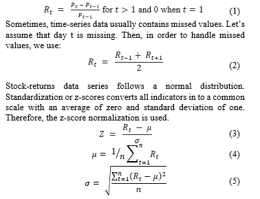
4. Piece wise Singular value decomposition (SVD)
The time series are usually good candidates for dimensionality reduction because they contain highly-correlated features [9]. To represent sequences, matrix is required. Singular value is a good feature of a matrix. It is feasible to use the SVD, when data follows a normal distribution [14] and also suitable for representing neighborhood. Therefore, the SVD is selected in this design. But, in order to reduce drawbacks of SVD, this paper introduces a novel approach to accomplish dimensionality reduction. This method is motivated by the simple observation that most of the time-series datasets can be approximated by segmenting the sequences into equal length sections and then recording the SVD of these sections, similar to the vectoring process used in PAA with mean value [9]. We can efficiently represent a “neighborhood” of data points with the reduced SVD value. These SVD values can be indexed efficiently in a lower dimensional space. This method can calculate SVD locally, and this new piecewise SVD removes the necessary of re-computing SVD for the entire dataset, when inserting to the clusters that we already have. Let us denote a time series query as and the set of time series of the dataset as . Let us assume that each sequence in Y is n units long (Previously, used filling value techniques for achieving this). Let N be the dimensionality of the transformed space that we wish to index . N may or may not be a factor of n. N being a factor of n is not a requirement of this approach. A time series X of length n can be represented in the N space by a vector . Let us take a nonnegative real number as the singular value for the matrix, generated by the vector . Then, the new reduced time series can be represented as . The ith element of W is calculated by the following equation:![]()
In simple terms, to reduce the time series from n dimensions to N dimensions, the data is divided into N equal sized “frames”. The SVD of the data falling within a frame is calculated and that is a nonnegative real number. The sequence of these values becomes the reduced time series representation.
5. Time series matching technique
In order to use with SVD, whole matching is selected. Here, since we are using the whole matching technique, as the previous original series, time series needs to be compared with all the other series in . After dimension reduction, the time series has been reduced to which has dimensions. Furthermore, all the other time series in the data set has been reduced to set of series with dimensions. Let us take all the other series in the reduced data set as and . Thus, to perform whole matching, one has to compare the reduced time series with the other time series in the data set . This comparison accomplished with measuring the distance as stated in the next section (III).
6. Distance Measure
For certain applications the Euclidean distance measure can produce notions of similarity which are very unintuitive. Thus, as a prototype, we use Euclidean distance measure. The Euclidean distance is a good “gold standard” [9] and BIRCH also supports Euclidean distance.
7. Time series clustering
In this research study, we propose clustering to identify dense and sparse regions in set of stock time series and, to discover overall distribution patterns and interesting correlations among stock time series [13]. Clustering can also be used for outlier detection. Alternatively, the proposed clustering method may serve as a preprocessing step for other algorithms, such as characterization; attribute subset selection, and classification, which would then operate on the detected clusters. Clustering can reduce a lot of time in selection of stocks as stocks of similar categories [26].
- Requirements of clustering:
First, it is required to identify the requirements of the proposed clustering algorithm. Since stock data are time-series data, be able to cluster time series data. Number of stocks is huge and volume of stocks is also large. Therefore, we need to find a method for efficient and effective cluster analysis of large datasets. Ability to handle outliers, minimal requirements for domain knowledge to determine input parameters, and ability to incorporate with newly inserted data into existing clusters are the requirements.
- Clustering algorithm – BIRCH
As described, BIRCH only stores CF vectors. CF vectors can be stored easily and can be calculated easily and accurately when merging. Storing CF vector is sufficient for clustering decisions [22]. Thus, BIRCH is good for a data set with lot of entries, such as a huge number of stocks. Furthermore, each entry in a leaf node is a sub-cluster, and not a single data point. Thus, the CF tree is a very compact representation of the dataset [22]. Therefore, BIRCH is suitable for a dataset with huge number of time series sequences.
Furthermore, the CF tree can be built dynamically, while inserting data. Therefore, BIRCH is very suitable for real-time, time-series big data clustering like in stock markets. Thus, future researchers can extend this research study to real time clustering [22]. Therefore, BIRCH which is used in this research is to give an efficient and accurate solution.
- Map Reduce
In order to give an efficient solution, parallel data processing technique is used. Therefore, Java Application Program Interface (API) of Hadoop MapReduce is selected for the implementation. Next section will discuss the implementation stage.
- Implementation
The implementation is divided into three main phases. The first phase involves in processing the time series, generating returns and data normalization. The second phase is to generate the reduced series. Clustering using BIRCH is the last phase. This phase generates clusters with the same trend, which can be used for further clustering using another method or can be used for further analysis process. Furthermore, clusters with single stock can be used for stock fraud detection.
Stock data from yahoo finance, during 1st of January 2000 and 30th of November 2016 were selected. Thus, Number of records per company is 6179 and Number of companies used is 9000. The data is in ‘metastock’ format.
Apache Hadoop MapReduce is used to achieve the parallelism of processing. Apache Hadoop Java API, Hadoop libraries, and Apache Mahout Libraries were used in the implementation. Next sections will describe the steps of the implementation.
First, filled missing values and then normalization process were implemented using java. Then as described in earlier sections, ‘piecewise SVD’ was implemented. Due to the local behavior of new piecewise SVD, it can effectively be used for parallel processing. This piecewise SVD removes the necessity of re-computing SVD for the entire dataset, when inserting the clusters that we already have. Thus, we only need to calculate the reduced series for the current insertion series. Then the clustering process was implemented. In order to accomplish the implementation of BIRCH, we modified the ‘jbirch’ implementation of ‘Roberto Perdisci’[1] according to our requirements. Next section will focus on evaluation and results.
- Evaluation And Results
This section evaluates the difference phases of the proposed approach based on comparisons, time complexity and visual analysis of results.
First, we focus on the novel dimensionality-reduction approach and time complexity of it. Let us take an example time series: closing prices of stock Aalberts Industries (AALB.AS). This series contains 4401 values and is shown in Figure 1. (Using the chart from Yahoo Finance to visualize easily)
Figure 1- Closing prices of stock Aalberts Industr (AALB.AS)
When using piecewise SVD and number of dimensions as 8, this time series is reduced to:
[532.6446625096315, 416.8873393376198, 930.5871525547732, 1102.8832536583386, 206.39692810698506, 325.16997582033906, 472.1037659773537, 663.7071469029098] and is shown in Figure 2.
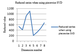
Figure 2- Closing prices of AALB.AS, when using piecewise SVD and 8 dimensions
In order to do a comparison, particular original series processed using piecewise aggregate approximation (PAA) with 8 dimensions. Results are:
[22.53275164735288, 17.36341740513517, 38.1274619404681, 39.638409452397134, 8.413749602363096, 13.765098841172463, 19.827730061349694, 28.209734151329258] and shown in Figure 3.
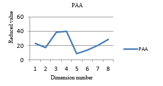
Figure 3- Closing prices of AALB.AS, when using PAA and 8 dimensions
When comparing two graphs (Figure 2 and Figure 3), both have much similar shapes.
Let us take the same time series: closing prices of stock AALB.AS. When using piecewise SVD and number of dimensions as 20, this time series has reduced to:
[332.3925127014745, 364.7341703213453, 290.44596055032366, 203.1714561644916, 297.2408049040378, 417.95588810303883, 591.8952354935798, 846.2187567644681, 891.780199993249, 214.3798407033649, 111.96008132365769, 125.80219373683428, 182.04229624732812, 216.06621785924793, 200.37451241363, 241.1271972942913, 331.1352621663843, 349.7118797667588, 426.1323476339242, 437.8459535327464] and shown in Figure 4.
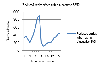
Figure 4- Closing prices of AALB.AS, when using piecewise SVD and 20 dimensions
In order to do a comparison, particular original series processed using PAA with 20 dimensions. Results are:
[22.284253578732113, 24.53078845716883, 19.513928652578947, 13.629266075891842, 19.782185866848458, 27.921654169506937, 39.799772778913876, 56.72833446943877, 55.645944103612784, 14.31897296069074, 7.061522381276979, 8.299890933878666, 12.191888207225627, 14.44708020904339, 13.446739377414218, 16.193206089525106, 22.225585094296747, 23.433946830265832, 28.684389911383786, 29.556532606225836] and shown in Figure 5.
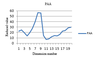
Figure 5- Closing prices of AALB.AS, when using PAA and 20 dimensions
When comparing two graphs (Figure 4 and Figure 5), both have much similar shapes but, piecewise SVD has a better gap between values with dimension number. Thus, this helps to give more accurate clusters in the clustering process. Further, when comparing Figure 3 and Figure 5, PAA has changed the shape of the graph, because PAA is ignoring the co-related behavior of values of time series. But, piecewise SVD remains the same shape, when comparing Figure 2 and 4. Thus, when using piecewise SVD, number of dimensions has reduced accurately. Therefore, this technique can be used to reduce stock time-series data. Furthermore, because of the new local behavior of SVD, can use this new piecewise SVD in the clustering process effectively. Effectiveness will be evaluated in the next section.
11. Evaluation of the time complexity
For full SVD, on an matrix A, , the time complexity is in [27]. Thus, when K is the number of stocks and n is the length of a time series, as the previous old method, time complexity is: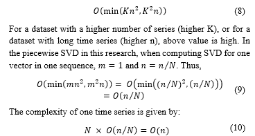
Computing reduced time series for different sequences are processed in parallel. Thus, there is no impact of in the piecewise SVD. Therefore, the piecewise SVD has a lower time complexity than the original SVD. Another major advantage of the piecewise SVD is the ability to perform SVD locally. As a result of using one time series at a time, we can perform SVD locally and thus, can add a new series to existing clusters without computing the SVD for the whole data set. Therefore, the local behavior removes the necessity of re-computing the SVD for the entire dataset, when inserting the clusters that we already have by adding a parallelization strategy.
12. Evaluation of the clustering
In most of the previous research approaches, the quality of the stock clustering and time-series clustering have been validated via visualizing the resulting clusters instead of statistical measurements [5,14,28,29,30]. The reason is that even though the statistical measurements give a numerical number, they cannot give accurate measurements. Thus, to assess how well this methodology clusters stock-market data, we performed a visual analysis of sets of stocks in the same groups and those in different groups. Yahoo Finance line charts were used to plot stock price movements of these stocks over the maximum period of available time, and the actual time period used in this research (i.e., Jan 1, 2000 to Nov 30, 2016) is visualized using a vertical line when needed.
Let us take a simple sample with 156 stocks from industry sector ‘American Express’ (AMEX). Here, the number of dimensions used is 8 and the distance threshold used is 20. Tickers of the final clustering results are:
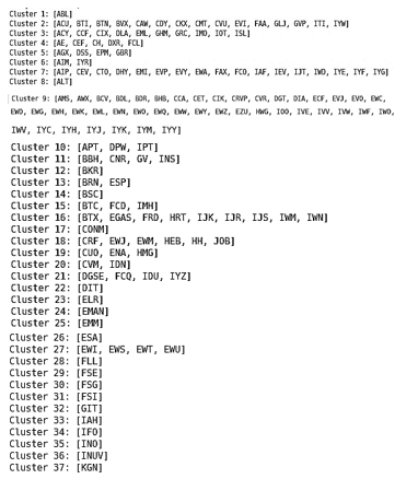
Figure 4- Final clustering results of a sample with 156 stocks from AMEX sector
Let us take closing prices and trends of some stocks of cluster 16, as an example. Graphs are taken from the current yahoo exchange pages of particular stock[1]. Blue line indicates the original closing prices of stocks. Also, in order to compare only the trend part, let us take simple moving averages of IJR, IWN, IJS and IWM stocks of cluster 16. The simple moving average is used to get the trend out of the stock-price time series. Thus, now, seasonal and irregular parts have been removed. Here, the green line is the simple moving average with 50 periods and the red line is the simple moving average with 100 periods, which indicates trends.
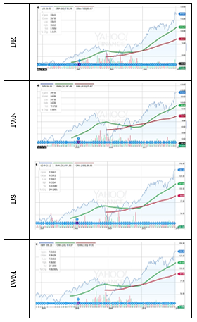
Table 1- Price curves and trend curves of cluster 16
Thus, according to the graphs of cluster 16, price curves of stocks of cluster 16 are much similar. Also, it shows that, the trend curves of same cluster stocks are same. Therefore, financial analyzers can use trend curves of stocks of a cluster to build a model of trend curves. Furthermore, it can be used to forecast stocks of that cluster, using models like Autoregressive Integrated Moving Average (ARIMA) models. Let us take some outliers, which are clusters with only one stock. Let us take simple moving averages of those outliers in order to compare only the trend part of outliers. Starting point of our data set is “Jan 1 ‘00”, which is indicated by a crossed horizontal and vertical line.
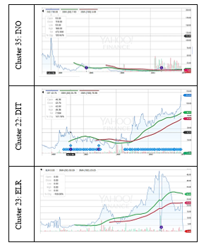
Table 2- Price curves and Trend curves of outliers
Thus, there exist a big different between shapes of price curves between outliers. For example, there is an abnormal behavior due to sudden downtrend in ELR of cluster 23. Thus, financial analyzers can further process outliers for fraud detection using price curves or trend curves. Furthermore, price curves of stocks of cluster 16 and price curves of outliers have a dissimilarity. Thus, from these stock price plots, it is apparent that the shapes of the same cluster price curves are similar, but there is a great difference in different clusters. The trend curves of outliers are different from other stock trends and can detect sudden decreases of trends like in ELR of cluster 23.
When the distance threshold increases, it can be got outliers far away from other clusters, which is good for further processing of fraud detection. When the distance threshold decreases, more refined clusters can be gained to receive accurate forecasting results.
13. Stress testing results
In order to give some indication about the running time of the program, running times with different number of stocks are listed below. Here, one stock is 6179 dimensions lengthier.
- Total time: Total running time in milliseconds
- CommittedVirtualMemorySize: The amount of virtual memory that is guaranteed to be available to the running process in bytes, or -1 if this operation is not supported.
- FreePhysicalMemorySize: The amount of free physical memory in bytes.
- FreeSwapSpaceSize: The amount of free swap space in bytes.
- ProcessCpuLoad: The “recent CPU usage” for the Java Virtual Machine process.
- ProcessCpuTime: The CPU time used by the process on which the Java virtual machine is running in nanoseconds.
- SystemCpuLoad: The “recent CPU usage” for the whole system.
- TotalPhysicalMemorySize: The total amount of physical memory in bytes.
- TotalSwapSpaceSize: The total amount of swap space in bytes.
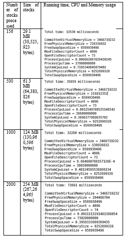
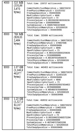
Table 3- Running time, CPU and Memory usage with different loads of stocks
Thus, according to these comparisons, it shows that this method can process massive data sets. Therefore, this method is suitable for process time series big data such as stock time series.
14. Conclusions and Future Work
In this paper, clustering method for time-series data based on SVD is proposed. The method takes advantages of the piecewise SVD and clustering to visualize efficiently the time-series data, which improves the processing efficiency and analysis of time-series data. We successfully implemented this method on Hadoop platform which provides the capabilities to process massive data. Furthermore, the real historical stocks are analyzed by this method on Hadoop platform: first, the data normalization, then, the feature extraction by piecewise SVD, and finally, the clustering by BIRCH with good results.
15. Conclusions
This research added a value to time series, data mining, and big data fields. First of all, this research explores a theoretical background related to time-series data. This can be seen as a case study to time-series mining research area. Very special decisions made in the stock data normalization phase can apply to time series data sets which follow a normal distribution. Furthermore, the novel piecewise SVD approach has numerous advantages than previous approaches. It is simple to understand and implement and can be applied to dimensionality reduction very accurately and efficiently. This will solve most of the problems with high-dimensionality and high-noisy in time-series data. Furthermore, the novel piecewise SVD has a local behavior, which is an opposite characteristic when considering the original SVD which has a global behavior. Therefore, this new piecewise SVD is suitable for big data. Furthermore, because of this local behavior, piecewise SVD can be used for parallel processing, and this piecewise SVD removes the necessity of re-computing the SVD for entire dataset, when inserting to the clusters we already have.
Previous stock and other time-series clustering methods have only succeeded with traditional clustering methods like k-means, canopy, AprioriAll, SOM, etc. This research concludes that, BIRCH is suitable for data distributions which have time-series behavior with high noise and high dimensions such as stocks and can be used to cluster massive time series data very accurately and efficiently.
Therefore, the overall methodology can be applied to process big time-series data with a normal distribution such as stocks in an efficient manner.
As stated in literature, the previous stock data clustering methods focused only on clustering the trend curve, because, it is very difficult to cluster the actual prices. But, in this research, the price curves of the stocks have clustered efficiently in an accurate manner. The first reason for this is that the correct methods used in the preprocessing stage, which was selected after a good study about time series data behaviors and stock data behaviors. The second reason is the novel approach of using SVD accurately with a local behavior.
Therefore, the method of this research can support exploratory search and facilitate serendipitous discovery. Besides revealing groups of similar stocks, this visualization can be used to find stocks that show different trading patterns. Such discovery can help traders to identify, for example, a set of hot stocks, stocks with a same trend and outliers and can further analysis of fraud detection or for forecasting. Instead of chasing the hot stocks, some investors may prefer to buy undervalued or oversold stocks. To find such stocks, they can explore clusters of stocks that have a sudden downtrend. This strategy may help financial analyzers to reduce the volatility of a portfolio and assist in decision-making process of buying and selling stocks. Therefore, this research enhances the prediction procedure of time-series data via an optimum clustering method.
Future directions
In order to identify subtle patterns with very short life times, Piecewise SVD will be extended for subsequent matching, instead of whole matching. Furthermore, future work should be continued to cluster data with different dimensions and should be continued to time series forecasting, with respect to particular data domains separately. Furthermore researchers can extend the methodology for different data distribution types, instead of normal distributions. Moreover, the researchers can extend this to real time stream processing using big data engine such as Spark because of BIRCH.
14. Conclusions and Future Work
- Hamed Davari Ardakani, Jamal Shahrabi Ehsan Hajizadeh, “Application of data mining techniques in stock markets: A survey,” Journal of Economics and International Financex, vol. Vol. 2(7), pp. pp. 109-118, July 2010.
- Ruey S. Tsay, Analysis of financial time series, Second Edition ed., Noel A. C. Cressie, Nicholas I. Fisher David J. Balding, Ed. Hoboken, New Jersey and Canada: A John Wiley & Sons, Inc., Publication, 2005.
- Dr. Samidha D. Sharma Abhishek Gupta, “Clustering-Classification Based Prediction of Stock Market Future Prediction,” (IJCSIT) International Journal of Computer Science and Information Technologies, vol. Vol. 5 , no. 3, pp. 2806-2809, 2014.
- Farhat Roohi, “Artificial Neural Network Approach to Clustering,” The International Journal Of Engineering And Science (Ijes), vol. 2, no. 3, pp. 33-38, 2013.
- Yung-Piao Wu and Hahn-Ming Lee Kuo-Ping Wu, “Stock Trend Prediction by Using K-Means and AprioriAll Algorithm for Sequential Chart Pattern Mining,” Journal of Information Science and Engineering, vol. 30, pp. 653-667, 2014.
- Sun Xin, “The application of Factor Analysis in Chinese Stock Market,” Collage of Science Tianjin Polytechnic University, Tianjin (300160), Research paper.
- Marco Aliotta, Andrea Cannata, Carmelo Cassisi, Alfredo Pulvirenti Placido Montalto, “Similarity Measures and Dimensionality Reduction Techniques for Time Series Data Mining,” in Advances in Data Mining Knowledge Discovery and Applications.: InTech, ch. 3, pp. 71-96.
- M.Punithavalli V.Kavitha, “Clustering Time Series Data Stream – A Literature Survey,” (IJCSIS) International Journal of Computer Science and Information Security, vol. 8, no. 1, pp. 289-294, April 2010.
- Kaushik Chakrabarti, Michael Pazzani, Sharad Mehrotra Eamonn Keogh, “Dimensionality Reduction for Fast Similarity Search in Large Time Series Databases,” Department of Information and Computer Science, University of California, Irvine, California 92697 USA, Research Paper 2000.
- J. Vargas, A. Pascual-Montano C.O.S. Sorzano, “A survey of dimensionality reduction techniques,” National Centre for Biotechnology (CSIC), C/Darwin, 3. Campus Univ. Autonoma, 28049 Cantoblanco, Madrid, Spain, Survey.
- Eric Postma, Jaap van den Herik Laurens van der Maaten, “Dimensionality Reduction: A Comparative Review,” Tilburg centre for Creative Computing, Tilburg University, 5000 LE Tilburg, The Netherlands, Review 2009.
- Imola K. Fodor, “A survey of dimension reduction techniques,” Center for Applied Scientific Computing, Lawrence Livermore National Laboratory, Livermore, survey 2002.
- Micheline Kamber Jiawei Han, “Cluster Analysis,” in Data Mining: Concepts and Techniques, Microsoft Research Jim Gray, Ed. San Francisco, CA 94111: Diane Cerra, 2006, ch. Chapter 7, pp. 383-466.
- Aziguli Wulamu, Yantao Wang, Zheng Liu Yonghong Xie, “Implementation of Time Series Data Clustering Based on SVD for Stock Data Analysis on Hadoop Platform,” 2014 9th IEEE Conference on Industrial Electronics and Applications , pp. 2007-2010, June 2014.
- Alexander Thomasian and Chung-Sheng Li Vittorio Castelli, “CSVD: Clustering and Singular Value Decomposition for Approximate Similarity Searches in High Dimensional Spaces,” IBM Research Division, Almaden, Austin, Beijing, Haifa, T.J. Watson, Tokyo, Zurich, IBM Research Report RC 21755 (98001), 2000.
- Aliaksei Sandryhaila, Jonathan Gross, Markus Doru Balcan, “Alternatives to The Discrete Fourier Transform,” Carnegie Mellon University, Pittsburgh, PA 1521, Survey 0634967,.
- Jon Wickmann, “A wavelet approach to dimension reduction and classification of hyperspectral data,” Faculty of Mathematics and Natural Sciences, University of Oslo, Oslo, Thesis 2007.
- J.R.G. & Barrios, E.B. Lansangan, “Principal components analysis of nonstationary time series data,” Statistics and Computing, vol. 19, no. 173, June 2009.
- Paul D. Gilbert and Erik Meijer, “Time Series Factor Analysis with an Application to Measuring Money,” University of Groningen, Research School SOM, Groningen, Research report 05F10, 2005.
- Jiri Dvorsky, Vaclav Snasel Pavel Praks, “Latent Semantic Indexing for Image Retrieval Systems,” Dept. of Applied Mathematics and Department of Computer Science, Technical University of Ostrava, listopadu, Ostrava – Poruba, Czech Republic, Research Paper.
- Pavel V. Senin, “Literature Review on Time Series Indexing,” Collaborative Software Development Lab, Department of Information and Computer Sciences, University of Hawaii, Honolulu, HI, CSDL Technical Report 09-08, 2009.
- Raghu Ramakrishnan, Miron Livny Tian Zhang, “BIRCH: An Efficient Data Clustering Method for Very Large Databases,” in SIGMOD ’96 6/96, Montreal, Canada, June 1996, pp. 103-114.
- Geeta Sikka Sangeeta Rani, “Recent Techniques of Clustering of Time Series Data: A Survey,” International Journal of Computer Applications (0975 – 8887), vol. Volume 52, no. No.15, pp. 1-9, August 2012.
- Keith Gutfreund, “Big Data Techniques for Predictive Business Intelligence,” in – (Held to be in future), -, 2015, pp. 64-70.
- Assoc. Prof. Dr. Sevtap Kestel, “Time Series Analysis – Classical Time Series,” 2013.
- B. Mahanty, M.K. Tiwari S.R. Nanda, “Clustering Indian stock market data for portfolio management,” Expert Systems with Applications, vol. 37, pp. 8793-8798, 2010.
- Alexander G. Gray, Charles Lee Isbell, Jr Michael P. Holmes, “Fast SVD for Large-Scale Matrices,” College of Computing, Georgia Institute of Technology, Atlanta, Research report.
- Joel Joseph and Indratmo, “Visualizing Stock Market Data with Self-Organizing Map,” in Proceedings of the Twenty-Sixth International Florida Artificial Intelligence Research Society Conference, Florida , 2013, pp. 488-491.
- Kate A. Smith, Rob Hyndman and Damminda Alahakoon Xiaozhe Wang, “A Scalable Method for Time Series Clustering,” School of Business Systems and Department of Econometrics and Business Statistics, Monash University, Victoria, Australia, Research paper.
- Vamsidhar Thummala, Kamalakar Karlapalem Vipul Kedia, “Time series forecasting through clustering – A case study,” International Institute of Information Technology, Hyderabad, India, Research paper.