1. Introduction

Diffraction means bending of electromagnetic waves from a sharp edge, wedge, corner and narrow slits. The diffraction takes place in the case of relatively higher wavelength of electromagnetic wave from obstacle or slit aperture. This paper is an extension of work originally presented in Electromagnetic wave theory symposium [1]. In case that wavelength of electromagnetic wave is less than the height of obstacle; high frequency asymptotic techniques are used [2]. Geometrical optics model runs for refraction, reflection, direct propagation and have been used for a long time in wave propagation in lit region. Geometrical optics model cannot explain diffraction concept [3], and thus cannot give accurate field prediction particularly behind an obstacle. In order to solve the diffraction problem in the field prediction, geometrical theory of diffraction (GTD) model is introduced [4]. However, GTD model gives inaccurate outcomes in optical boundaries [5]. GTD gives inaccurate results in the situation that source, diffraction and observation points are in the same line [6].  GTD model is an extension to geometric optic model by adding diffracted fields terms and used in high frequency spectrum [7]. UTD model is introduced in order to overcome singularity problem of GTD model [8]. UTD model gives appropriate and exact outcomes in case of single diffraction [5]. UTD model is also an extension to geometric optic model and reflected waves are also considered in field prediction [6]. UTD model gives inaccurate outcomes in field prediction in the situation of closer building height. In order to predict the field strength more exactly, the second order diffracted field terms are added to total field at the receiver [9]. Slope diffraction model is introduced in [10, 11]. However, there are some singularities in field prediction at shadow boundary points [12]. Higher order diffraction coefficient and diffracted fields are developed to predict the relative path loss at the receiver for wedge and knife edge structures [13-15]. Amplitude and slope diffraction coefficients are developed via providing amplitude, slope and phase continuities in optical boundaries [16]. Slope UTD model applied multi-shaped cascaded obstacles [17] and adapted into time domain and all formulas are derived in time domain [18]. A new GTD model is introduced for equal heights case [19]. After 10 diffractions slope UTD model loses the accuracy and requires more computation time. S-UTD-CH model is proposed to predict the field strength accurately after 10 diffractions for knife edge and wedge structures [20, 21]. Amplitude and slope diffraction coefficients are used in S-UTD-CH model developed in MATLAB environment. Firstly location and height data of transmitter, obstacle and receiver is entered to program. And then a ray tracing is made and all contribution to total path loss at the receiver is determined. Afterwards, by using amplitude and slope diffraction coefficient path loss is calculated. As an example a simple test scenario is used in order to show that effect of diffraction coefficient is maximum in case of plane angle diffraction. All the simulations are performed in MATLAB.

2.       Amplitude Diffraction Coefficient

To calculate the total field behind an obstacle formula [8] is given by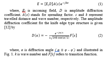

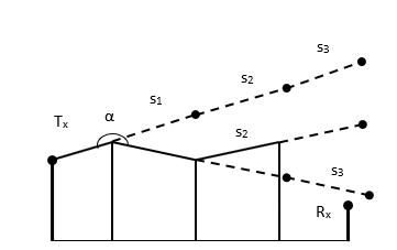
Fig.1. Multiple Knife edge Diffraction Scenario

Amplitude diffraction coefficient used in calculation of the diffracted fields behind the obstacle. The amplitude diffraction coefficient changes with respect to diffraction angle. The diffraction angle is measured between incoming and diffracted fields as depicted in Fig. 1. Changing of the amplitude diffraction coefficient with regard to diffraction angle is shown in Fig. 2.

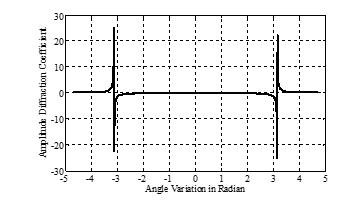
Fig. 2. Amplitude diffraction coefficient vs diffraction angle

As it is seen in Fig. 2, the diffraction angle variation is indicated on horizontal axis. Variation of the amplitude diffraction coefficient is indicated on vertical axis. Also it can be seen in Fig. 2, the magnitude of amplitude diffraction coefficient has the maximum value at π and – π radian (180° and -180°). Plane angle diffraction takes place in the case that source, diffracting and observation points are in the same line.

3.       Slope Diffraction Coefficient

In order to calculate the diffracted field behind multiple obstacles, slope diffraction coefficient have to be used to predict the field strength accurately. The slope diffraction coefficient can be calculated by the formula [12] expressed by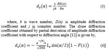

where, k is wave number, L_s is distance parameter for slope diffraction coefficient and F[x] refers to transition function.

Slope diffraction coefficient used in calculation of the diffracted fields behind multiple obstacles. The slope diffraction coefficient changes according to the diffraction angle. Again the diffraction angle is measured between incoming and diffracted fields as depicted in Fig. 1. UTD model fails in predicting of the diffracted field in case of equal or closer obstacle height. In order to remove the discontinuities in the predicted field, derivatives of the amplitude diffracted fields have to be added on the receiver. Changing of the slope diffraction coefficient with respect to diffraction angle is shown in Fig. 3.

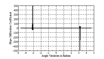
Fig. 3. Slope diffraction coefficient vs diffraction angle

As it is seen in Fig. 3, the diffraction angle variation is indicated on x-axis. Variation of the amplitude diffraction coefficient is indicated on y-axis. Also it can be seen in Fig. 3, the magnitude of the slope diffraction coefficient has the maximum value at π and – π radian (180° and -180°). By adding the slope diffracted fields, the deficiency of UTD model in equal height case is removed [22-23].

If there are 3 or more obstacles in the propagation scenario, normal derivative of the slope diffraction coefficient have to be used in prediction [12] is given by,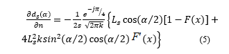

where, k is wave number, s is travelling distances, is L_s is distance parameter for slope diffraction coefficient and F[x] refers to transition function. Also F՛[x] is derivative of transition function.

Derivative of the slope diffraction coefficient used in calculation of the diffracted fields behind multiple obstacles, when the obstacle number is greater than 2. The derivative of the slope diffraction coefficient changes with the diffraction angle. Again the diffraction angle is measured between incoming and diffracted fields as depicted in Fig. 1. Changing of the derivative of the slope diffraction coefficient with respect to diffraction angle is shown in Fig. 4.

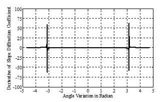
Fig. 4. Derivative of slope diffraction coefficient vs diffraction angle

As it is seen in Fig. 4, the diffraction angle variation is indicated on abscissa. Variation of the amplitude diffraction coefficient is indicated on ordinate. Also it can be seen in Fig. 4, the magnitude of the slope diffraction coefficient has the maximum value at  and –  radian (180° and -180°).

4.  Results and Discussion

In order to verify the contribution of diffraction is maxima in the plane angle diffraction, test scenario in Fig. 5 is used.

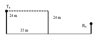
Fig. 5. Plane angle test scenario

As it is depicted in Fig. 5, the transmitter antenna height is 24 m, obstacle is 35 m apart from the transmitter and whose height is 24 m. Operating frequency is 300 MHz.  Path loss variation for direct and diffracted fields with respect to the receiver height just behind the obstacle (36 m) is illustrated in Fig. 6

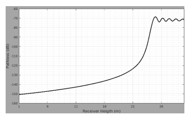
Fig. 6. Path loss of direct and diffracted fields together

As can be seen in Fig. 6, diffraction effect is maxima in the plane angle diffraction case. As the receiver height is 24 m, the angle between transmitter and receiver becomes 180°. After this height of receiver, direct field is dominated.

Path loss variation for only diffracted fields with respect to the receiver height just behind the obstacle (36 m) is illustrated in Fig. 7.

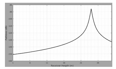
Fig. 7. Path loss of diffracted fields

As can be seen in Fig. 7, the diffraction effect is maxima in the plane angle diffraction case. As the receiver height is 24 m, the angle between transmitter and receiver becomes 180°.

Path loss variation for reflected and diffracted fields with respect to the receiver height just behind the obstacle (36 m) is illustrated in Fig. 8.

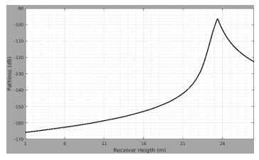
Fig. 8. Path loss of reflected and diffracted fields together

As can be seen in Fig. 8, diffraction effect is very much on the receiver position. In that position ground reflected fields make some contribution to total field. If the receiver height is increased the diffracted field contribution is decreased.

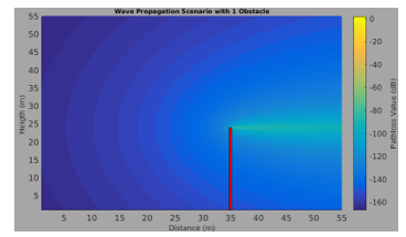
Fig. 9. Coverage Map

Furthermore, a coverage map is generated by using the simple test scenario in Fig. 5. By using only diffracted field, a coverage map is indicated in Fig. 9.

As it is seen in Fig. 9, the diffraction contribution is maxima in the case of plane angle diffraction. Plane angle diffraction takes place in the case that the receiver height is 24 m.

5.       Conclusions

The diffraction mechanism is significant to predict the field strength and it is used for coverage prediction in urban, rural and indoor environment behind an obstacle like rooftop, edge, corner, and vertex. This field generated by direct, reflected and diffracted waves.  The diffracted fields take place in the case of that wavelength of the electromagnetic wave is close or greater than the slit. In order to solve the diffraction problem in shadow region, a lot of electromagnetic wave propagation models are presented, such as GTD, UTD, S-UTD and S-UTD-CH. Amplitude and slope diffraction coefficient directly affect the total electromagnetic fields at the receiver. As the diffraction angle is close to plane angle, the contribution of slope diffracted field is so high. In the case of diffraction angle π radian; in other words observation, diffraction and field points are in the same line, contribution of amplitude and slope diffraction coefficient is maximum. In future, amplitude and slope diffraction coefficient will be developed for rectangular type structure.

Acknowledgment

This work is supported partially by TÜBİTAK (The Scientific and Technological Research Council of Turkey) under the grant no. 215E360.

1. M.B. Tabakcioglu, “Amplitude and Slope Diffraction Coefficients for S-UTD-CH Mode”, Electromagnetic Theory Symposium, Espoo, Finland, pp. 768-771, 2016.
2. C.A., Balanis, C.A., Advanced Engineering Electromagnetics. John Wiley & Sons, 981 p, New York, USA, 1988.
3. P.Y., Ufimtsev,  Fundamentals of the Physical Theory of Diffraction, John Wiley & Sons, 329 p, New Jersey, USA, 2007.
4. J.B., Keller, “Geometrical Theory of Diffraction”. J. Opt. Soc. Amer., vol. 52, no 2, pp. 116-130, 1962.
5. R.J. Luebbers, “A Heuristic UTD Slope Diffraction Coefficient for Rough Lossy Wedges”, IEEE Trans. Antenna Propagation.,vol. 37, no 2, pp. 206-211, 1989.
6. R.J.,  Luebbers, “Finite conductivity uniform GTD versus knife edge diffraction in prediction of propagation path loss”. IEEE Trans. Antennas Prorpagat, vol. 32, pp. 70-76, 1984.
7. C.A., Balanis, L. Sevgi, L. P.Y. Ufimtsev, “Fifty years of High Frequency Diffraction”, International Journal of RF and Microwave Computer-Aided Engineering, vol. 23, no. 3, pp. 394-402, 2013.
8. R.G.Kouyoumjian, P.H. Pathak, “A uniform geometrical theory of diffraction for an edge in a perfectly conducting surface”, Proceedings of the IEEE, vol. 62, pp. 1448–1461, 1974.
9. R.Tiberio, R. R.G. Kouyoumjian, “An analysis of diffraction at edges illuminated by transition region fields”, Radio Science, vol. 17, no. 2, pp. 323-336, 1982.
10. J.B. Andersen, “Transition zone diffraction by multiple edges”,  IEEE Proceedings  Microwave Antennas and Propagation, vol. 141, no. 5, pp. 382-383,1994.
11. H. Wang, “Modeling and Wideband characterization of Radio wave propagation”, Ph.D. Thesis. The University of Texas at Austin, Austin, USA, 2005.
12. C. Tzaras, S.R. Saunders, “An improved heuristic UTD solution for multiple-edge transition zone diffraction”, IEEE Transactions on Antennas and Propagation, vol. 49, no: 12, pp. 1678–1682, 2001.
13. P.D. Holm, “UTD-Diffraction Coefficients for Higher Order Wedge Diffracted Fields”,  IEEE Transactions on Antennas and Propagation, vol. 4, no: 6, pp. 879-888, 1996.
14. P.D. Holm, “A new heuristic UTD Diffraction Coefficients for nonperfectly conducting wedges”, IEEE Transactions on Antennas and Propagation, vol. 48, pp. 1211-1219, 2000.
15. P.D. Holm, “ Calculation of Higher Order Diffracted Fields for Multiple-Edge Transition Zone Diffraction”, IEEE Transactions on Antennas and Propagation, vol. 52, no:5, pp.1350-1355, 2004.
16. K. Rizk, R. Valenzuela, D. Chizhik, F. Gardiol, “Application of the slope diffraction method for urban microwave propagation prediction”, IEEE Vehicular Technology Conference, pp. 1150-1155, Canada, 1998.
17. G.Koutitas,  C. Tzaras, “A Slope UTD Solution for a Cascade of Multishaped Canonical objects”,  IEEE Transactions on Antennas and Propagation, vol. 54, no: 10, pp. 2969-2976, 2006.
18. A. Karousos, C. Tzaras, “Multi Time-Domain Diffraction for UWB Signals”, IEEE Transactions on Antennas and Propagation, vol. 56, no: 5, pp. 1420-1427, 2008.
19. A. Tajvidy, A. Ghorbani, “ A New Uniform Theory-of-Diffraction-Based Model for the Multiple Building Diffraction of Spherical Waves in Microcell Environments”, Electromagnetics, vol. 28, no: 5, pp. 375-387, 2008.
20. M.B. Tabakcioglu, A. Kara, “Comparison of improved slope UTD method with UTD based methods and physical optic solution for multiple building diffractions”, Electromagnetics, vol. 29, no:4, pp. 303–320, 2009.
21. M.B.Tabakcioglu,  A. Kara. “Improvements on Slope Diffraction for Multiple Wedges”, Electromagnetics, vol. 30, no: 3, pp. 285-296, 2010.
22. M.B.Tabakcioglu, D. Ayberkin, A. Cansiz,  “Comparison and Analyzing of Propagation models with Respect to Material, Environmental and Wave Properties”, ACES Journal, vol. 29, no:6, pp. 486-491, 2014.
23. M.B. Tabakcioglu, “S-UTD-CH model in multiple diffractions”, Internetional Journal of Electronics, vol. 103, no: 5, pp. 765-774, 2016.

(Click to view)

(Click to view)