Spatial Sampling Requirements for Received Signal Level Measurements in Cellular Networks of Suburban Area
Spatial Sampling Requirements for Received Signal Level Measurements in Cellular Networks of Suburban Area
Volume 2, Issue 1, Page No 277-287, 2017
Author’s Name: Abdlmagid Baserea), Ivica Kostanic
View Affiliations
Department of Electrical and Computer Engineering, Florida Institute of Technology, Melbourne, FL 32901, USA
a)Author to whom correspondence should be addressed. E-mail: abasere2011@my.fit.edu
Adv. Sci. Technol. Eng. Syst. J. 2(1), 277-287 (2017); ![]() DOI: 10.25046/aj020134
DOI: 10.25046/aj020134
Keywords: Coverage area estimation, Received signal level, Coverage verification in cellular systems

Export Citations
A process for the determination of a required spatial resolution in the collection of the Received Signal Level (RSL) is discussed. This method considers RSL measurements as a three dimensional surface that is sampled through the data collection process. In addition, it is difficult to collect RSL measurements for an entire coverage area because of many obstacles, for example, buildings, lakes, and vegetation. Thus, the estimation of the coverage area is necessary for locations for which it is hard to collect the RSL. Kriging is a well-known technique for estimation of unknown values at specific locations, and it has shown very good results. The distance factor in Kriging has never been studied before for a coverage area. A drive test is used to collect RSL measurements, and they are gathered in different distance sizes, a procedure is known as binning, to form the coverage area. Kriging is used to estimate the entire RSL surface in bin sizes that are 200×200, 100×100, 50×50, and 25×25 meters of resolution. Using a 2-D Fourier analysis, the cutoff frequency for the Fourier transform of the RSL surface is determined. The spatial sampling resolution and the cutoff frequency are linked through a Nyquist sampling criterion. The approach was experimentally verified in a typical suburban environment. The results show that the spatial resolution requirement is between 50 and 100m.
Received: 30 December 2016, Accepted: 23 January 2017, Published Online: 28 January 2017
1. Introduction
The cell coverage area is one of the most essential factors in cellular communication system designs [1, 2]. It can be defined as the greatest distance that a cell-phone can be away from the base-station while still receiving a reasonable service [3]. The base station is normally located near the center of the required served area [4].
In cellular networks, the coverage area of a cell is based on the signal strength of its pilot channel. For instance, in the case of a GSM cell, the strength of its Broadcast Control Channel (BCCH) needs to be over the suitable coverage threshold [5]. Also, in W-CDMA, the coverage depends on the signal strength of the Common Pilot Channel (CPICH) [6]. However, in LTE the convenient metric is the Reference Sequence Received Power (RSRP) [7]. While the system is deployed, the coverage area of every cell is tested through a procedure usually referred to as drive testing. This procedure includes measurement of the RSL of the pilot channel within the geographic area that surrounds the cell. Normally, the measurements are conducted using appropriate drive test receivers. These receivers pair measurements of RSL of the pilot channel with the geolocation information. The coverage area of the cell is estimated based on these measurements.
There are two principal practical issues with the RSL measurements. The first issue is associated with signal fading in the wireless environment. It is well understood that as a result of multipath propagation, the measured signal experiences small scale fading. Therefore, estimates of the RSL need to be obtained through some form of statistical averaging of the instantaneous signal readings. The process followed in the averaging of the instantaneous measurements needs to be compliant with a requirement frequently referred to as the Lee criterion. The requirement is described in [8, 9].
The second issue involves coverage area estimation. There are two aspects regarding this issue. First, in every practical scenario, the data may be collected only from a small portion of the area that is accessible to drive testing. Therefore, the coverage estimate for the entire area of interest is obtained through the process of measurement interpolation. An effective way for interpolation that is based on the Kriging method is presented in [1]. However, to make a valid interpolation, the measured data need to be sampled at a sufficient spatial resolution. To the authors’ knowledge, the issue of spatial sampling of the RSL has not received sufficient treatment in the available literature, and it is the subject of the work presented in this paper.
1.1. Cell Coverage Area
A cellular system network consists of cells that are linked together to offer radio coverage over a wide geographical area. The cell phone coverage area lets a large number of users communicate with each other, whereas base stations in the cellular network are stationary. These base stations provide a connection to transceivers regardless of their movement, whether they are stationary or moving across cells. The range of cell coverage is based on natural factors, for example, human factors, such as the landscape (urban, suburban, rural), subscriber behavior, and propagation conditions, etc. [10].
1.2. Importance of Understanding Cell Coverage Area
1.2.1. Coverage Planning
The coverage planning process can be divided into three phases. The first phase is named the preplanning phase. The general properties of the future network are examined. In the second phase, a site survey is used to examine the targeted area and an investigation of potential base stations’ locations is achieved. Following the initial survey, constant modification is necessary to move the network planning forward. In the last phase, a driving test to collect data is done repeatedly in order to test the coverage area until achieving good coverage. Then, the system is ready to be deployed in the target area to provide service [11].
1.2.2. Concept of Handoff
Handoff is a procedure that allows mobile users to move from one cell to another without interruption of service. The handoff process performance depends on a variety of conditions such as signal strength and interference levels [12]. Having an accurate picture of the coverage in a given region is necessary condition for reliable handoffs.
1.2.3. Interference
Interference results when neighboring cells simultaneously work on the same frequency. One of the main weaknesses that can limit the implementation of a cellular system in a multi-cell network is inter-cell interference. Interference can cause background noise and bad voice quality when a call is in operation. As a result, the determination of coverage area is beneficial in reducing the interference, which leads to higher quality of service [13].
1.2.4. User Location
The mobile telecommunication network consists of several base stations (BSs) that provide mobile telecommunication service to mobile users. Each BS represents a cell that is offering coverage to a specific area, and each cell is divided into sectors. Understanding the coverage of the sectors assists in locating the users that are within the systems of the service area [14].
1.3. Methods for Estimating Cell Coverage
There are many methods of performing the estimation of cellular coverage areas, and each of them has its own advantages and disadvantages, but none of them is 100% accurate [15]. Three implementation estimation methods are explained as follows.
1.3.1. Geometry
The algorithms that use Voronoi diagrams to estimate coverage areas do not take into consideration the features of the propagation environment, and they oversimplify the coverage problem [16]. For this reason, among others, Voronoi diagrams are not being used in this work.
1.3.2. Prediction
Coverage prediction and propagation modeling are among the most fundamental tasks in cellular system design. Over many years a diverse of methods have been used for coverage area prediction using propagation models. These models are useful in predicting path loss or signal attenuation, so they thus enable appropriate reception [17]. Cellular designers generally use advanced planning tools for estimating the network coverage. The estimation of coverage area is dependent on terrain data combined with a propagation model [18].
1.3.3. Measurements
A drive test is usually used to collect the RSL measurements. Performing driving tests is expensive and time consuming, so there have been significant attempts to improve the quality of coverage estimation for locations for which the values are unknown by using values that are obtained from a limited number of driving test measurements. The difficulty with drive tests is that data cannot be collected for the entire region of the network because of many barriers [18] such as lakes, vegetation, and buildings. Therefore, the estimation of the coverage area is significant and must rely on spatial prediction methods for instance, Inverse Artificial Neural Networks, Distance Weighting, and Kriging.
2. Problem Statement
The problem of spatial sampling of the RSL is demonstrated with the assistance of Figure 1. As shown in the figure, the RSL for a specified transmitter site might be seen as a three dimensional surface. During the procedure of data collection, one makes measurements of the “surface height” at different locations in space – i.e. different (x, y) coordinates. The job of interpolation is to reconstruct the surface on the basis of the collected measurements.
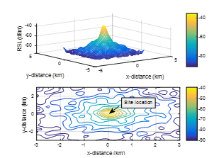
Figure 1: An illustration of the RSL surface
It is clear that the precision of interpolation is basically based on the spatial sampling “frequency” of the measurements. As the number of measurement locations becomes larger, the accuracy of the estimate for the RSL surface becomes higher. Yet, as with any sampling process, the point of diminishing returns is reached.
The objective of the study in this paper is to calculate the required spatial sampling rate for accurate representation of the RSL surface. Shannon’s sampling theorem is extended to a two dimensional signal representing the RSL surface in this analysis.
3. Literature Review
3.1. Data Collection
To verify the coverage area of the cellular system it is required that the RSL measurements be conducted by doing spatial averaging of immediate signal power measurements. The data is normally gathered in accordance with Lee sampling criteria. The amplitude of the received signal envelope in the mobile propagation environment is described in equation (1) [9].![]()
It is sensible to indicate the received signal by a stationary stochastic process, where denotes the variation of fast fading of a mean signal strength value equal to 1. The mean value of the signal envelope is , and is the location of the local mean [8].
Getting an estimation that is valid statistically for the local mean, there are two questions that need to be answered. First, how many ‘snapshots’ of the RSL are required to be conducted over an appropriate distance to make certain the statistical validity of the estimate. Second, what would be a suitable spatial distance to average over. Averaging the space over a distance has to be achieved to guarantee averaging Rayleigh fading effects. Estimation of the local mean can be considered as an average of the power of the signal over a suitable distance ( 2L ) as displayed in equation (2) [19]: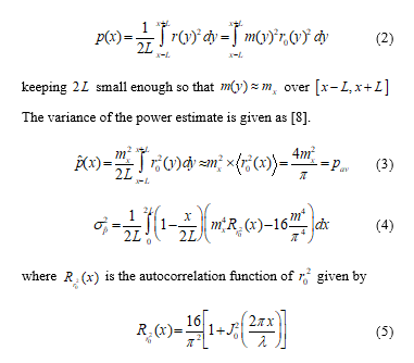
Equation (4) has been statistically evaluated [2] for different values of , and the results for and spreads are shown in Table 1 [19].
Table 1. Spread of the local mean estimate as a function of the averaging distance
| Spread | Spread | ||
| 2.98 dB | 6.5 dB | ||
| 2.14 dB | 3.5 dB | ||
| 1.55 dB | 3.24 dB | ||
| 1 dB | 2.1 dB |
Under most practical conditions, terrain variations (shadowing) over a distance can be presumed to be insignificant and can be considered as negligible. Therefore, the claim that the mean value of the signal is not variable during the integration in equation (3) is valid [19].
“Macroscopic propagation models predict the mean received signal level over a small geographical area called a bin” [19]. The size of the bin is computed as a function of accuracy, computation time, roughness of the terrain, and database terrain resolution, etc. Typically the size ranges from 50m to 500m. The local area mean (LAM) is the mean of the received signal of a bin. Playing averaging of several local means may allow comparison between measurement data with predictions of the propagation model [19].
While driving through a specific bin, the measurement equipment performs the collection of the local means within the bin. The local means tend to comply with a normal distribution in the logarithmic domain with a standard deviation and mean value . The local area mean for the particular bin is calculated as an average value of the local means collected in that specific bin.
where is the local area mean, represents the local mean and is the total number of local means collected in the bin [19].
3.2. Spatial Binning
Spatial binning is grouping of measurements that are close to each other. The binning results in a smaller geographically referenced data set, where each point represents an average obtained over a bin area [20].
Incomplete drive test data can cause imprecise estimation of coverage area. Yet, collection of excessive data is time consuming and costly. Grouping measurements using averaging can help reduce the processing load and quantify data to the resolution of a specific terrain which constitutes the bin of the area [19].
3.3. Interpolation Methods
Through interpolation, one-use measurement data samples can be collected and used to estimate measurement data at other points where measurement data are not available. Included in the most common spatial interpolation methods are spline interpolation, interpolating polynomials, Inverse Distance Weighting (IDW), and Kriging [21]. Amongst those techniques, Ordinary Kriging (OK) and IDW are the most frequently used, and are normally the most commonly suggested interpolation methods [22].
“Kriging is an interpolation technique based on the methods of geostatistics” [23]. Krige in 1951 collected samples over mining fields. The method was used as a optimal interpolation techniques to use in the mining industry. Currently, the Kriging method is being used in groundwater modeling, soil mapping [24, 25], and in several other spatial problems [24].
4. Proposed Application
4.1. Kriging Method
The principle of interpolation equation in the Kriging model is given by [23].
where is the known value at the location, is an unknown weight for the known value at the location, and is the estimation value.
As can be seen, at the point where the algorithm performs the interpolation, the value is obtained as a weighted average from the points in the immediate neighborhood. The most important mission linked with the implementation of (7) is the calculation of the appropriate weights. The fitted variogram model is used to determine the weights that are essential for local estimation. The interpolation may be unbiased by choosing the weights . Interpolating many locations may give some values that can be above and below the real values. Therefore, the summation of weights must be equal to 1 in order to ensure that the estimation of unknown values is unbiased [24].
4.1.1. Semivariogram
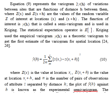
“The variogram characterizes the spatial continuity or roughness of a data set. Usually, one dimensional statistics for two data sets might be equal” [23]. Yet, the spatial continuity could be unrelated. The difference between the variogram and the semivariogram is just a factor of 2. The semivariogram equation (9) is described in [24].![]()
he nugget, the range, and the sill, as shown in Figure 2. experimental semivariogram offers beneficial information for optimizing sampling, interpolation, and determining spatial patterns. It is obvious that the number of semi-variogram values is proportional to the pairs of locations. In addition, when datasets are large, the number of pairs of locations will increase quickly. As a result, the binning of the distance is necessary to obtain the variogram parameters, which are the range, the nugget, and the sill [24]. Moreover, in the case of RSL interpolation, the binning of the data is important so that the results of fast fading can be reduced.
4.1.2. Fitting Variogram Models
The fitting model is determined by plotting the empirical semivariance versus the separation distance of the pairs of locations (lag distance) [27], so the relationship between them provides specific parameters, namely t
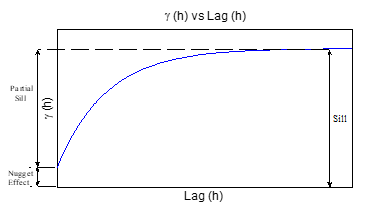
Figure 2: Simple transitional variogram with range, nugget, and sill
A variogram model is a parametric curve fitted to a variogram estimator. There are several semivariogram fitting models that are used in the Kriging method to help estimate data precisely, and the most commonly used semivariogram models are summarized in Figure 3 [24]:
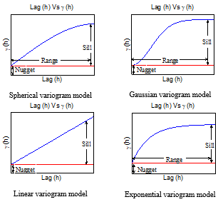
Figure 3: Examples of most commonly used variogram models
The remainder of this paper is organized as follows: Section V gives an overview of experimental verification, which is divided two parts. In the first part the measurement setup, data collection, and results of interpolation are presented, and the second part has a discussion of the Fourier Spectrum of the RSL surface, and the verification of the approach for determining required sampling distance. In Section VI, a brief summary and conclusions are provided.
5. Experimental Verification
The collection of RSL measurements was performed in an area that is located in Melbourne, FL. The map of the area is presented in Figure 4. Although the study is conducted on a specific RF frequency, the methodology should be widely applicable across all UHF/VHF frequencies used for personal communication systems. The Melbourne area is a suburban area. For the study, the transmitter is located on the rooftop of a multi-story building, making for good wide area coverage. The majority of houses in the targeted area are one to two floors, and their heights range from 4 to 9 meters. Also, there are open areas such as small artificial lakes, parks, and vegetation. The satellite view of the study area is shown in Figure 4.
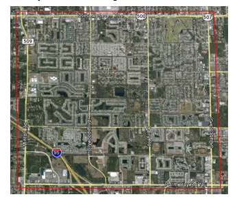
Figure 4: Satellite view of the studied environment
5.1. Experimental Verification For RSL Interpolation
5.1.1. Data Collection
An illustration of the data collection system is presented in Figure 5. The system consists of the following parts:
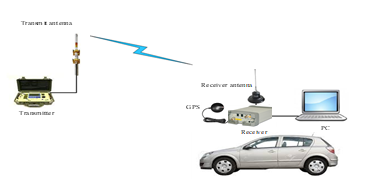
Figure 5: Illustration of the measurement system
- Transmitter: The transmitter is used to evaluate PCS band signal propagation, and the frequency range is 1.85 to 2.1 GHz, where the power is up to 43 dBm. This transmitter allows the transmission of the signal at the radio frequency of 1925MHz.
- Transmit Antenna: The transmitter antenna is used in the transmission of signals to be measured. It is an omnidirectional antenna, and its frequency ranges between 1850 MHz and 1990 MHz. It also radiates in a horizontal plane with 6 dBi gain.
- Receiver: An Agilent Technologies E6474A receiver is used to conduct RSL measurements at different spatial locations.
- Receiver Antenna: The receiver antenna is used to collect RSL measurements. It is an omnidirectional antenna with a frequency range between 1850 and 1990 MHz.
- GPS Antenna: The GlobalSat BU-353-S4 is a USB magnet mount GPS receiver. Its characteristics are low power consumption, an ultra-compact chipset, and extreme sensitivity. It is appropriate for marine navigation, mobile phone navigation, automotive navigation, and personal positioning. It can be connected with a PC in order to allow JDSU Wireless Solutions software to recognize and store the location of measured data in terms of longitude, latitude, and altitude. The recorded position enables the user to get the best interpolation of the coverage area.
5.1.2. Data Collection and Binning
A drive test was undertaken in the selected geographic area, where RSL measurements were collected and stored. The RSL measurements are collected to perform estimation for gaps as shown in Figure 6.
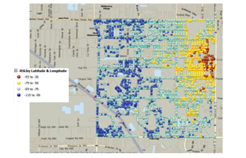
Figure 6: View of the studied environment and measured data
The RSL measurements are used to produce a coverage area map for the targeted area. Every spatial location can be defined as a point of intersection of both the x-axis and the y-axis, where the x-axis represents the longitude and the y-axis represents the latitude. A Matlab code is used to perform the binning. Since the data set is large, the binning is done for the coverage area as shown in Figures 7-10 with different resolutions. The binning is based on a separation of adjacent bins, such as 25×25, 50×50, 100×100, and 200×200 meters.
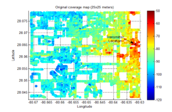
Figure 7: Original coverage area of 25×25 meters resolution
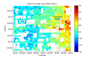
Figure 8: Original coverage area of 50×50 meters resolution
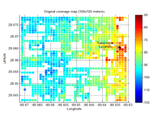
Figure 9: Original coverage area of 100×100 meters resolution
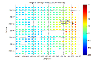
Figure 10: Original coverage area of 200×200 meters resolution
The semivariogram of the fitting model can be determined by plotting the empirical semivariogram versus the distance as shown in Figure 11. It shows that as the dataset becomes large, the number of observations will increase quickly.
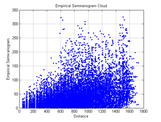
Figure 11: Empirical semivariogram cloud
The difficulty in the computation of the semivariogram fitting model increases as the size of the dataset increases. As a result, the points of the variogram cloud can be grouped into classes of distances (“bins”) to get the variogram fitting model for the area of interest. The RSL measurements demonstrate that the variogram fitting model is linear as shown in Figure 12.
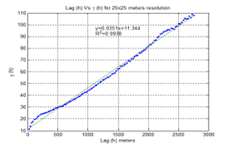
Figure 12: Linear variogram model of 25×25 meters resolution
5.1.3. Data Collection and Binning
The interpolation result of the targeted coverage area for grid sizes of 25×25. 50×50, 100×100, and 200×200 meters resolution are shown in Figures 13-16. The interpolation of the coverage area with 25×25 meters resolution is smooth, and it gives more details about the RSL as shown in Figure 13.
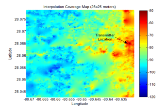
Figure 13: Interpolated coverage area of 25×25 meters resolution
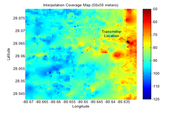
Figure 14: Interpolated coverage area of 50×50 meters resolution
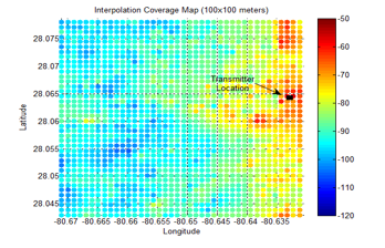
Figure 15: Interpolated coverage area of 100×100 meters resolution
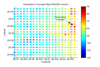
Figure 16: Interpolated coverage area of 200×200 meters resolution
5.2. Experimental Verification For Determining Required Sampling Distance
5.2.1. Fourier Spectrum of The RSL Surface
The two dimensional Fourier analysis is used, with the 2-D spectrum of the RSL surface represented as: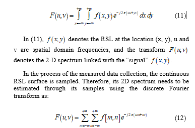
In (12), shows the RSL measurement conducted at the location and, and are sampling distance increments in x and y direction from the transmitting site.
As in any practical application, the RSL surface spans only the finite portion of the x-y plane; and the summation in (12) is performed over a finite amount of samples. This leads to a 2-D spectrum given by: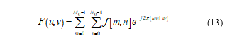
The 2-D spectrum in (13) captures all the frequency components participating in the formulation of build up of the “signal” . The spatial sampling results in the periodic extension of the signal’s 2-D spectrum. The spatial frequency of the sampling process needs to be sufficiently high so that the aliasing between the spectrum replicas is negligible.
As a further clarification, consider the 2-D magnitude spectrum, i.e. , associated with the RSL surface shown in Figure 1, and presented in Figure 17. The RSL is sampled over a 6km by 6km area with the sampling distances m and m. The spectrum in Figure 17 is generated after the DC component of is removed. The plot in Figure 2 reveals that the RSL surface is a low pass 2-D signal and that one may establish the highest frequency in its 2-D spectrum – . The contribution of the spectral terms that are above the highest frequency of the overall energy of becomes negligible. Hence, based on the well-known Nyquist sampling criterion, the sampling frequency needs to be at least two times , and the maximum sampling distance in the x-y plane is given as:
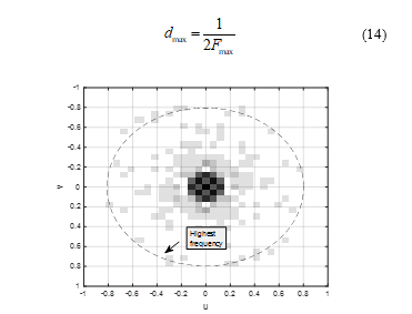
Figure 17: 2D-Spectrum associated with the RSL surface given in Figure 1
Therefore, to determine the furthest sampling distance required for sampling of the RSL surface, one may follow the following procedure:
- Perform sampling of at the smallest possible distance increments and that are guaranteed to satisfy the requirement given in (14).
- Use a low pass filter to determine the largest significant frequency in the spectrum of the sampled signal, . Once the largest significant frequency is determined, the maximum sampling distance in the spatial domain is given by (14).
Following the above outlined procedure faces several obstacles. Firstly, the value of is directly related to the variability of the RSL caused by the log normal shadowing. The log normal shadowing is environmentally dependent and therefore becomes environmentally dependent as well. Therefore, the initial sampling needs to be done at a fairly fine grid that guarantees that the criterion in (14) is satisfied. Secondly, the measurement can never be collected over the entire area of interest. Therefore one needs to rely on the interpolation to generate a best estimate of the entire RSL surface. This topic is discussed in [1]. Finally, one needs to establish a criterion for determination of . By eliminating all the spectrum components outside of the circle in Figure 17, a fraction of the energy is eliminated as well. As a result of this elimination, a filtered version of the 2-D spectrum is obtained as: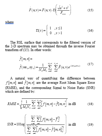
where is the average RSL over the complete area of attention. The SNR in (19) based on . As decreases, additional high frequency components from the 2-D spectrum are removed. Therefore, the RMSE in (18) rises and thus the SNR in (19) decreases. Based on the study reported in [28], the RSL measurements are repeatable within 3dB. In this study, the difference between and that is a result of filtering in (15) is considered as a random variable. The highest significant frequency is computed so that the absolute value of this difference is below 3dB in more than 95% of points.
5.2.2. Verification of The Approach for Determining Required Sampling Distance
The data are collected with a spatial resolution of 25m. In other words, over the drive test route, a measurement is stored each 25m. It is supposed that this resolution is higher than what would be required by the condition in (14). Moreover, as it may be seen, the data are collected over all locations available for drive testing – i.e., every road in the area is tested.
Baseline Received Signal Level Map: From the measured data shown in Figure 6, a baseline of RSL surface is created. The baseline surface has a bin resolution of 25 by 25 m. The interpolation procedure depends on the Kriging technique explained in [1]. The baseline map generated through the interpolation is shown in Figure It is considered as an accurate representation of the RSL surface.
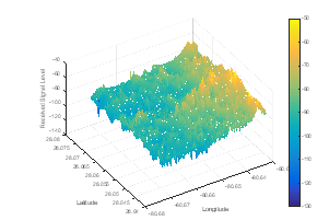
Figure 18: Baseline RSL surface obtained from data in Figure 3 through Kriging interpolation
The algorithm shown in Figure 19 is applied to determine the maximum frequency in the spectrum of the RSL surface. The interpolated RSL surface is transferred into the frequency domain through a 2D Fourier transform. The Fourier spectrum of the surface is low-pass filtered as shown in Figure 17. A filtered version of the spectrum is brought back into the spatial domain through the inverse 2D Fourier transform, and the performance metrics as defined in (18) and (19) are generated. The results of the process are summarized in Table 2. The table shows the following columns:
-
- represents the normalized low pass cut off frequency. The initial sampling of the RSL surface through the drive test process is performed at a resolution of 25m. Therefore, the sampling distance m and the sampling frequency is m-1.
- The average RMSE is calculated on the basis of (18).
- 95% of RMSE – Difference between filtered RSL surface and the baseline RSL surface at a given point may be treated as a random variable. The value reported in this column is the 95% percentile of the estimated cumulative distribution. In other words, 95% of the points exhibit absolute difference smaller that the value reported in this column.
- The average SNR is calculated using (19).
sampling distance is calculated as .
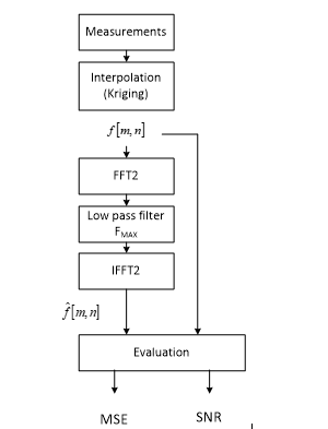
Figure 19: Algorithm for determination of the maximum frequency in the RSL surface spectrum
As expected, a larger sampling frequency results in a smaller MSE and a larger SNR. At the same time, a larger results in a more frequent sampling of the RSL surface in the spatial domain. For example, the value of yields a filtering frequency of which corresponds to the sampling distance of 83 meters. This sampling distance introduces an average RMSE of roughly 1.68dB and the 95% value of 2.43dB. The SNR of the approximation is on the order of 13.93dB.
Table 2. Values of MSE and SNR as a function of the filtering frequency
| Average RMSE (dB) | 95% of RMSE (dB) | SNR (dB) | (m) | |
| 0.2 | 2.42 | 3.75 | 10.52 | 125 |
| 0.3 | 1.97 | 2.92 | 12.45 | 83 |
| 0.4 | 1.68 | 2.43 | 13.93 | 63 |
| 0.5 | 1.47 | 2.16 | 15.10 | 50 |
| 0.6 | 1.30 | 2.00 | 16.22 | 42 |
| 0.7 | 1.14 | 178 | 17.34 | 36 |
| 0.8 | 0.98 | 1.58 | 18.65 | 31 |
| 0.9 | 0.80 | 1.27 | 20.43 | 28 |
Based on the values in Table 2, and the study in [28], the choice of seems to be appropriate. This choice corresponds to the sampling distance of 83m and the 95% value of 2.92dB, which is within the bounds of the RSL measurement repeatability.
6. Summary and Conclusion
The RSL measurements were collected in a suburban area. The interpolation of the coverage area for a targeted area was done successfully. Measurements demonstrate that the semivariogram fitting model is linear. The use of Kriging confirms the interpolation to be very efficient. It provides a good result when the coverage area is divided into different bin sizes that are 25×25, 50×50, 100×100, and 200×200 meters of resolution. Furthermore, the importance of exact RSL measurements for the binning process is shown. The approach seems to be promising and is expected to be worth pursuing at a larger scale.In this study, the Shannon sampling theory was used to determine the appropriate spatial sampling distance in the RSL measurements. It is explained that the RSL surface can be treated as a two-dimensional low pass signal for which a maximum cutoff frequency can be recognized. By means of this experimental work, a cutoff frequency was determined for a typical suburban environment in the US. The value of in the measured environment was 0.006 1/m and the value for the corresponding sampling distance is 83m.In general, the corresponding sampling distance and the cutoff frequency are functions of the propagation environment. It is expected that environments with higher variability of the path loss, i.e., with more pronounced lognormal shadowing, have a higher value of Thus, the sampling distance in such environments needs to be smaller than the one obtained in this work. Similarly, for environments that are less variable than the suburban environment in this study, the value of should be smaller, and correspondingly, a coarser sampling in the spatial domain may be preferable. For future attempts, a study that establishes an value and corresponding sampling distance across various propagation environments may be undertaken.
- Basere and I. Kostanic, “Cell Coverage Area Estimation From Receive Signal Level (RSL) Measurements,” World Congress on Engineering and Computer Science (WCECS), 2016, in press.
- Basere and I. Kostanic, “Spatial Sampling Requirements for Received Signal Level Measurements in Cellular Networks,” IEEE Computing and Communication Workshop and Conference (CCWC), 2017, in press.
- Jiang and C. H. Davis, “Cell-coverage estimation based on duration outage criterion for CDMA cellular systems,” IEEE transactions on vehicular technology, vol. 52, pp. 814-822, 2003.
- D. Parsons and P. J. D. Parsons, “The mobile radio propagation channel,” 2000.
- M. Redl, “An Introduction to GSM,” Atech House Publishers, 1995.
- Holma and A. Toskala, WCDMA for UMTS, 3rd Ed., Wiley 2004.
- Dahlman and S. Parkvall, 4G: LTE.LTE-Advanced for Mobile Broadband, Accademic Press, 2011.
- C. Y. Lee and Y. S. Yeh, Ón the Estimation of the Second-Order Statistics of Log-Normal Fading in Mobile Radio Environment,” IEEE Transaction on Communication, Com-22, June 1974, pp. 869-873.
- Kostanic, J. Zec and N. Faour, “Sampling Criteria for Wideband Received Signal Measurements,” in proc. of International Conference in Wireless Networks, Las Vegas, NV, June 2003, pp. 24-29.
- K. Sharma and R. Singh, “Cell coverage area and link budget calculations in GSM system,” International Journal of Modern Engineering Research (IJMER) vol, vol. 2, pp. 170-176, 2012.
- Sun, “Radio Network Planning for 2G and 3G,” Master of Science in Communications Engineering, Munich University of Technology, 2004.
- R. Manoj, “Coverage estimation for mobile cellular networks from signal strength measurements,” Citeseer, 1999.
- -S. Sheu and W.-H. Sheen, “Characteristics and modelling of inter-cell interference for orthogonal frequency-division multiple access systems in multipath Rayleigh fading channels,” IET Communications, vol. 6, pp. 3015-3025, 2012.
- Arigela, P. Veerendra, S. Anvesh, and K. Satya, “Mobile Phone Tracking & Positioning Techniques,” International Journal of Innovative Research in Science, Engineering and Technology, vol. 2, 2013.
- Akbari, O. Onireti, M. A. Imran, A. Imran, and R. Tafazolli, “Effect of inaccurate position estimation on self-organising coverage estimation in cellular networks,” in European Wireless 2014; 20th European Wireless Conference; Proceedings of, 2014, pp. 1-5.
- Argany, M. A. Mostafavi, F. Karimipour, and C. Gagné, “A GIS based wireless sensor network coverage estimation and optimization: A Voronoi approach,” in Transactions on Computational Science XIV, ed: Springer, 2011, pp. 151-172.
- Sharma and R. Uppal, “RF Coverage Estimation of Cellular Mobile System,” Intrnational journal of Engineering and Technology, vol. 3, p. 60, 2011.
- Sayrac, J. Riihijärvi, P. Mähönen, S. Ben Jemaa, E. Moulines, and S. Grimoud, “Improving coverage estimation for cellular networks with spatial bayesian prediction based on measurements,” in Proceedings of the 2012 ACM SIGCOMM workshop on Cellular networks: operations, challenges, and future design, 2012, pp. 43-48.
- Kostanic, N. Rudic, and M. Austin, “Measurement sampling criteria for optimization of the Lee’s macroscopic propagation model,” in Vehicular Technology Conference, 1998. VTC 98. 48th IEEE, 1998, pp. 620-624.
- Hoeber, G. Wilson, S. Harding, R. Enguehard, and R. Devillers, “Visually representing geo-temporal differences,” in Visual Analytics Science and Technology (VAST), 2010 IEEE Symposium on, 2010, pp. 229-230.
- Zimmerman, C. Pavlik, A. Ruggles, and M. P. Armstrong, “An experimental comparison of ordinary and universal kriging and inverse distance weighting,” Mathematical Geology, vol. 31, pp. 375-390, 1999.
- Li and A. D. Heap, “A review of comparative studies of spatial interpolation methods in environmental sciences: Performance and impact factors,” Ecological Informatics, vol. 6, pp. 228-241, 2011.
- Konak, “Estimating path loss in wireless local area networks using ordinary kriging,” in Proceedings of the Winter Simulation Conference, 2010, pp. 2888-2896.
- A. Burrough, R. A. McDonnell, R. McDonnell, and C. D. Lloyd, Principles of geographical information systems: Oxford University Press, 2015.
- Kbiob, “A statistical approach to some basic mine valuation problems on the Witwatersrand,” Journal of Chemical, Metallurgical, and Mining Society of South Africa, 1951.
- Wackernagel, Multivariate geostatistics: an introduction with applications: Springer Science & Business Media, 2013.
- K. Leung and T. Law, “Kriging Analysis on Hong Kong Rainfall Data,” HKIE Transactions, vol. 9, pp. 26-31, 2002.
- Mijatovic and I. Kostanic, “Repeatability of Received Signal Level Measurements in GSM Cellular Networks”, in proceedings of 2nd International Symposium on Wireless Pervasive Computing, Feb 2007.