Real Time Implementation of an Improved Hybrid Fuzzy Sliding Mode Observer Estimator
Real Time Implementation of an Improved Hybrid Fuzzy Sliding Mode Observer Estimator
Volume 2, Issue 1, Page No 214-226, 2017
Author’s Name: Sorin Mihai Radu1, Elena-Roxana Tudoroiu2, Wilhelm Kecs2, Nicolae Ilias1, Nicolae Tudoroiu3,a)
View Affiliations
1Mechanical and Electrical Engineering Faculty, Mechanical Engineering, University of Petrosani, 332006, Romania
2Science Faculty, Mathematics and Informatics, University of Petrosani, 332006, Romania
3John Abbott College, 2127 Lakeshore Road, Sainte-Anne-de-Bellevue, QC, H9X 3L9, Canada
a)Author to whom correspondence should be addressed. E-mail: ntudoroiu@gmail.com
Adv. Sci. Technol. Eng. Syst. J. 2(1), 214-226 (2017); ![]() DOI: 10.25046/aj020126
DOI: 10.25046/aj020126
Keywords: Fuzzy Sliding Mode Observer, Fault Detection and Isolation, Residual Generation, Dc Servomotor Angular Speed

Export Citations
This paper extends some of our research results disseminated in the most recent awarded international conference paper concerning the implementation in real time of a sliding mode observer state estimator. For the same case study developed in the conference paper, more precisely a DC servomotor angular speed control system, we extend the proposed concept of sliding mode observer state estimator to a fuzzy sliding mode observer version, more suitable in control applications field such as fault detection of the possible faults that might take place inside the actuators and sensors. The hybrid architecture implemented in a real time MATLAB/SIMULINK simulation environment consists of an integrated control loop structure with a switching bench of two sliding mode observers, one built by using a new approach that improves slightly the proposed sliding mode observer for the conference paper, and second one is an improved intelligent fuzzy version sliding mode observer estimator. The both estimators are implemented in SIMULINK to work independently by using a manual switch. The simulation results for the experimental setup show the effectiveness of the improved fuzzy version of sliding mode observer compared to the standard one, as well as its high accuracy and robustness.
Received: 18 December 2016, Accepted: 20 January 2017, Published Online: 28 January 2017
1. Introduction
This paper is an extension of the results disseminated in the most recent international conference paper relating to the real time implementation of a sliding mode observer (SMO) state estimator, integrated in a direct current (DC) servomotor angular speed control system [1]. The main goal of the extended version paper is to investigate new directions for improving the SMO state estimator performance in terms of state estimation accuracy and robustness to the changes in the noise levels, initial conditions values of the estimates, input disturbance and modeling errors uncertainties. The improved version of the SMO estimator is a fuzzy version of SMO (FSMO), a real helpful tool for our future developments in the real time control applications field, namely several real time fault detection and isolation (FDI) control strategies based on various estimation techniques. The purpose of these FDI strategies is to detect and isolate the possible malfunction components inside the actuators and/or faulty sensors as vital control system components frequently prone to errors. The real-time simulations are carried out on the MATLAB/SIMULINK platform, that has special real time implementation features provided by its extensions Real-Time Workshop (RTW) and the Real-Time Windows Target (RTWT). Furthermore, the real-time dc servomotor angular speed control proposed in our case study can be easily interfaced with MATLAB/SIMULINK or Any Logic multi-paradigms hybrid simulator in the case of Real-Time Unified Modeling Language (UML-RT) implementations with a fast response [2]-[4].
2. Fault Detection and Isolation Schemes Using Real Time State Estimators
The DC servomotor is mostly used as an actuator in feedback closed-loop control systems, but in this research for simulation purposes it is considered in the same time as a controlled plant, similar with the one shown in Figure 1 [2]-[4]. One of the main goals of this closed-loop structure might be to control its angular speed or its position either or both. Nowadays, the DC servomotors are extensively used in the common control applications due to their high start torque characteristics, high response performance, and their speed much easier to be controlled by varying the input voltage, compared to those that need expensive frequency drivers [1].
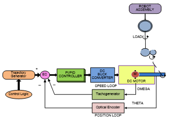
Figure 1: The schematic diagram of the closed-loop control system of the dc servomotor angular speed (Reproduced from [4]).
The components of the DC servomotor actuators during operation experience several possible critical failures that could compromise its performance and cause severe gear damage, such as, armature coil opening, brushes failures, field coil opening, armature static converter short circuit, field static converter short circuit, armature coil short circuit, field coil short circuit, cooling system failure, lack of bearings and bushing lubrication, armature current sensor failure, field current sensor failure, offset on supplied voltage or speed sensor failure [5].
Whenever these critical situations come out the control systems could lose the control, require much more energy, and could operate harmfully. Therefore to operate in real-time at high energy efficiency and to guarantee the equipment safety and reliability it is important to develop suitable FDI strategies capable to detect and diagnose any time every faulty control system components and consequently corrective and reconfiguration actions should be initiated promptly [1]. Fault detection and isolation schemes are implemented as real-time algorithms based on various state estimation techniques that require the input-output measurements data set of the control plant. They are basically used firstly for fault detection to decide whether the plant is in a normal operating condition or in a faulty one, and secondly for fault isolation to point out and identify the kind of the fault, if it is present, among a given faults covering set [1], [5]. Effectively the existing methods to identify and to adjust the equipment failures are mostly labor-intensive task, and consequently sustained, rhythmic and error-prone [1]. In the most of these situations the windings currents are recorded to determine the health of the DC servomotors currents compared to statistical evaluation that necessitates considerable human knowledge, hence error-prone that could generate severely equipment operation [1]-[6]. In these conditions the problem of control systems monitoring and fault diagnosis becomes a critical issue, of high complexity that need to be implemented in real-time environment by using more sophisticated control systems and artificial intelligence estimation strategies [1]. Usually, the control systems design must include FDI issues at their very early design stage with the ultimate goal to reach a fault-tolerant control (FTC) environment [5], [7]. Following the FDI diagnosis, on-line procedures are usually needed for FTC purpose, while off-line procedures could be used for maintenance purpose [5], [7]. To see the strong link between the FDI real time algorithms and the state estimation techniques is worth to know that a FDI strategy is implemented as a two-steps procedure based on the plant data set of input-output measurements. In the first real time procedure step is implemented the fault detection or is generated an alarm to decide whether the system is in a normal operating condition or not using an estimation algorithm, such as Kalman filters estimators [6], [8]-[9] or Luenberger linear and nonlinear sliding mode observers [10]-[16]. In our approach we develop a hybrid structure for state estimation, namely a fuzzy version of sliding mode observer nonlinear estimator, FSMO similar to the approach developed in [17]-[18]. In the second procedure step the isolation tasks or alarms interpretation are required for right decision about which faults chosen from a pre-defined set of faults that cover almost all the possible situations (fault isolation) [5], and therefore to find the faults locations based on an implemented logic, as in our future extension approach (second part of this research paper) that will develop for this purpose an intelligent fuzzy logic classifier [10]. The set of output measurements along with a previously obtained knowledge of the system constitute the
algorithm inputs while a set of generated alarms are the algorithm outputs [5]. It is also worth to say that accuracy and the robustness of these estimation techniques are crucial for successful real time implementation of all FDI strategies. Furthermore, these estimation techniques are useful to establish the fault characteristics such as occurrence time, its severity, and the recovery time. The FDI estimation algorithms performance is the ultimate analysis issue that must consider also the accumulate evaluation errors included at every step of the FDI problem solution. This research work is based on our previous experience in control systems implementation, very useful to prove the effectiveness of the improved version of real-time SMO estimator implementation, a simple fuzzy version, FSMO. It will be a new practical approach to build a hybrid control structure that integrates in the same control loop the FDI control strategy together with a FSMO estimator and a fuzzy logic classifier (FLC). Summarizing, the main objective of this research is to improve the performance of the real time SMO estimator developed in the most recent paper conference [1] using a new approach. The new SMO estimator design is an improved fuzzy version of SMO estimator, very simple to be implemented in real-time, more efficient, accurate, robust and consistent. The improved FSMO estimator is a useful tool capable to be applied in our future developments in control applications field, as an extension of these research results to find solutions for different control applications, such as for example the most attractive FDI control strategies.
3. Dynamics Model of Dc Servomotor
For simulations purpose to implement our proposed real time FDI strategy of actuator (input) and sensor (output) faults we consider the same permanently excited DC servomotor with a rated power of P = 550 W at rated speed n = 2500 rpm, described in detail in [7]. It consists of two-pair brush commutation, two pole pairs, and an analog tachometer for speed measurement and operates against a hysteresis brake as load, as shown in Figure 2 [7].
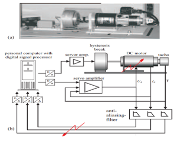
Figure 2: The Dc servomotor test bench with hysteresis brake
a) The experiment set-up b) The equipment block scheme (screenshot from [7])
The measured signals of the angular speed control system are the armature voltage , the armature current and the angular speed . The closed-loop equipment includes in forward path an analog proportional servo amplifier and the dc servomotor actuator as a controlled plant. In the feedback path is integrated an analog tachometer transducer, three anti-aliasing filters (AFs), three Analog to Digital converters (ADC) as an interface between an input personal computer (PC) and the AF block, a second analog servo amplifier with pulse-width-modulated (PWM) armature voltage as output and speed and armature current as feedback that allows to be built a cascaded speed control system [7]. In Figure 2(b) is shown the flow diagram of the three measured signals that first pass through analog anti-aliasing filters and after they are processed by a digital signal processor (e.g. TXP 32 CP, 32-bits, 50 MHz) and a desktop Intel Pentium host PC [7]. Also the hysteresis brake is controlled by a pulse-width servo amplifier. Typically such dc servomotors can be described by linear dynamic models [1], [7], [20].
However, the simulation results of the experiments carried out have shown that these linear models with constant parameters do not match the process in the entire operational range [7]. For that reason, the block scheme of dc servomotor represented in complex domain must include two nonlinearities such that the dynamic model is capable to capture all the process dynamics, as is shown in Figure 3 [7]. The dynamics of the dc servomotor actuator is described by the following input-state-output equations [1], [20]: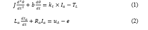
where is the dc servomotor torque developed on the shaft, is the load torque, is the magnetic flux, as is shown in Figure 3 and Table 2 [7]. In addition by defining the armature voltage as , as is shown in Figure 3, and the DC servomotor counter electromotive force, e by:
where represents a two-norm bounded noise vector which stands for the uncertainties and the unknown inputs affecting a practical DC servomotor [7].
Output equation![]()
The measurement vector, is assumed to be completely known and measurable at each sample time, t. The unknown disturbance, is bounded, i.e. there exists a positive real value, such that the symbols ||.|| and stand for the two-norm of noise vector and the upper bound value of , respectively.
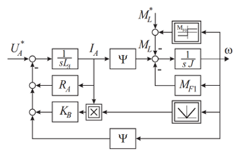
Figure 3: The block scheme of the Dc servomotor in complex domain (screenshot from [7])
3.1. Abbreviations and Acronyms and measure units
To simplify the presentation we include in this subsection the list of all the abbreviations and the acronyms used in the paper text, as is shown in Table 1.
Also in the text we use only the international standard (SI) as primary units, as is shown in Table 2
Table 1: The list with the abbreviations and the acronyms used in text
| Item |
Acronyms/ Abbreviations |
Significance |
| 1 | FDI | Fault Detection and Isolation |
| 2 | FTC | Fault Tolerant Control |
| 3 | PC | Personal Computer |
| 4 | PWM | Pulse-Width-Modulation |
| 5 | AF | Anti-aliasing Filter |
| 6 | ADC | Analog to Digital Converter |
| 7 | SMO | Sliding Mode Observer |
| 8 | FSMO | Fuzzy Sliding Mode Observer |
| 9 | FIS | Fuzzy Inference System |
| 10 | FLC | Fuzzy Logic Classifier |
| 11 | KF | Kalman Filter |
| 12 | RTW | Real Time Workshop |
| 13 | RTWT | Real-Time Windows Target |
| 14 | UML-RT | Real Time Unified Modeling Language |
| 15 | SI | International System of Units |
| 16 | DC | Direct Current |
Table 2: The list with the SI units abbreviations used in the text
| Name | Symbol | SI base Unit | Expressed in other SI units | Name of SI unit |
| Current | I | A | – | ampere |
| Voltage | V | V | – | volt |
| Time | t | s | – | second |
| Magnetic flux | ψ | Wb | weber | |
| Viscous friction coefficient (Damping ratio of the mechanical system) | – | – | ||
| Moment of rotor inertia | – | – | ||
| Dry friction coefficient |
– |
– |
||
| Counter electromotive force coefficient | ke ψ |
– |
Nm/A |
– |
|
Electromotive force |
e |
V |
– |
volt |
| Proportional coefficient of the motor torque | kt ψ |
Nm/A | – | |
| Electric resistance of the armature | Ω | Ohm | ||
| Electric inductance of the armature | H | Ω s | Henry | |
| Angular speed | – | – | ||
| Load torque | – | – | ||
| Motor torque | – | |||
| Electric Power | W | watt |
The nominal values of the DC servomotor model coefficients have the same values as in [7], as are given in Table 3.
Table 3: The nominal values of the dc servomotor dynamic model
| Parameter Name | Symbol | Value | Measure Unit |
| Electric resistance of the armature | 1.52 | Ω | |
| Electric inductance of armature |
H ( Ωxs) |
||
| Magnetic flux | ψ | 0.33 |
Wb ( |
| Voltage drop factor | KB | ||
| Moment of rotor inertia | |||
| Viscous friction coefficient | |||
| Viscous dry friction | 0.11 |
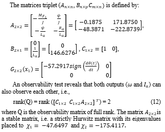
Replacing the values given in Table 3 in the dc servomotor dynamic model represented by (4)-(6) we get the nominal system equations of the dc servomotor dynamics in a state space representation of the following form: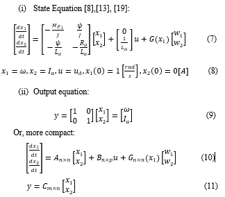
where n represents the system state dimension, n = 2, p is the number of inputs, p = 1,and m is the number of outputs, m = 2. The load torque is considered as a bounded input uncertainty included in the last term, of (7). The noise vector components are generated by a SIMULINK “Band-Limited White Noise” block that generates normally distributed random numbers that are suitable for use in continuous or hybrid systems of different spectral density powers, e.g., 1 and 0.1 to analyze also the robustness of the hybrid structure SMO – FMSO estimators to the different noise levels.
4. Sliding Mode Observer for Linear DC Servomotor with Model and Disturbances Uncertainties
Basically the design of any SMO estimator for a nonlinear uncertain system can be simplified by considering its linearized model, similar to those described by (10)-(11), proposed for sate estimation and written in the following most general form [7]: 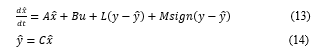
where, the estimated state vector is denoted by , and is the residual of the output signal of the control system. L represents an appropriate designed linear gain matrix, similar to Luenberger Observer gain matrix for linear systems [11], [13] [18] and M is an appropriate designed nonlinear gain matrix that multiplies the common sign function, as in [1] and [16], [18]. In reality they represent two key tuning parameters to control the SMO performance. In Equation (13) its last term is added to compensate the effects of disturbance input (load torque) and modeling uncertainty of the system (10). Therefore, the states of the system can be estimated using data given by the measured input-output data set, of the control system. Several design methods have been used to determine the observer linear gain L, ensuring the stability of the proposed SMO estimator [18]. Among these design methods in [18] is mentioned the most popular Kalman Filter (KF) algorithm that can be applied to find the estimation gain as a good approximation of the gain matrix L for the designed SMO linear estimator (13). Closing, the proposed SMO linear estimator (13) includes two key terms: one of them is the Kalman filter term as a suitable approximation of the Luenberger observer term, , and the other one is the discontinuous sign term, , where their corresponding gains and are designed separately [18]. Therefore, the proposed observer design (6) becomes the mixed Kalman Filter – SMO estimator (KF-SMO), whose dynamics is described by the following single input-single output (SISO) output equation: ![]()
![]()
By some manipulations of the matrices we can easily find that have a full rank, and also the pair we found in section 2 that is observable, as main requirements assumed in [14]-[16], [18].
By replacing (16) in (15), the dynamics of SMO observer is described by the following equation [18]:![]()
where the matrix concentrates all the dynamics of SMO estimator, so it has to be stable (strictly Hurwitz) such that the state estimate, to converge to a finite value in a finite time [14]-[16], [18]. The matrix is strictly Hurwitz if all its eigenvalues are situated strictly in the half left complex plane, The dynamics of the SMO estimator (15) is described by the following first order differential equations: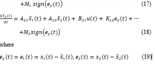
represent the states residuals of the DC servomotor. The observer linear gain matrix is chosen in order to make the spectrum of the matrix ( to lie in [14]-[16], [18]. In simulations we consider two cases, one case for eigenvalues close to origin of the complex plan, for a slow transient, and second case for eigenvalues far from origin of the complex plan, for fast transient, very important in fault detection. Without to lose the generality we can select for the sliding mode observer the following linear gain matrices, setting the matrix components as and for any value greater than -0.1875 that guarantees the stability of the matrix ( , e.g.,![]()
We analyze in this case the accuracy of the hybrid structure SMO-FSMO estimators corresponding two different poles locations of control system, given as the eigenvalues of the matrix . The main goal remains now to design the nonlinear gain matrix M such that the discontinuous term, overcomes the parametric uncertainties assuring a stable dynamics of SMO estimator error. The observer nonlinear gain matrix has to guarantee a bounded error dynamic for the output residuals (19) satisfying the following gain condition [18]:
![]()
Also the gain condition (20) assures that the SMO residuals converge to zero. More precisely, the two-norms of the known term G(x) and the SMO gain matrix M are bounded to corresponding upper bounds, and respectively [18].According to (20) taking into account the noise levels for gain matrix M we will consider in our simulations the following values 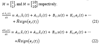
4.1. Sliding Mode Observer Simulation Results
For simulation results purpose in the experimental set-up the input voltage profile is set to in the first 0.5 seconds and to on the last 0.4 seconds. Also the spectral density power values of the noise will be set in first case to 1 and for second case will be chosen ten times smaller to 0.1 in order to be able to see the accuracy of the both estimators SMO, and FSMO, The problem design of the sliding mode observer is solved by using one of the most powerful tools, such as MATLAB/SIMULINK software package.
The SIMULINK model of the nominal system is shown in Figure 4, and the evolution of the DC servomotor states, i.e. angular speed and armature current are shown in Figure 5 and Figure 6. The input profile voltage is shown in Figure 7. In Figure 8 is presented in detail the DC servomotor subsystem nominal model. In Figure 9 is shown the overall view of the SMO SIMULINK diagram of the state estimator. The Figure 10 and Figure 11 show the dynamic evolution of the SMO armature current residual and on the same graph the both model and SMO armature current estimate. Similar for SMO angular speed is shown in Figure 12 and Figure 13. In Figure 14 is shown the switch control function on the sliding surface, to analyze the chattering effects of the sliding mode on the control system efforts to keep the evolution of the states on the trajectory.
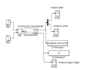
Figure 4: The overall SIMULINK diagram of DC servomotor nominal model
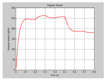
Figure 5: The MATLAB simulations of the evolution of nominal DC Servomotor angular speed
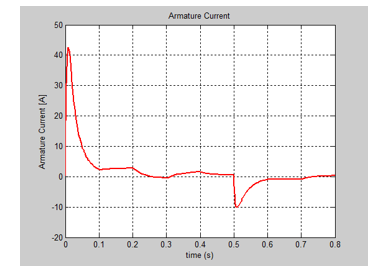
Figure 6: The MATLAB simulations of the evolution of nominal DC Servomotor armature current
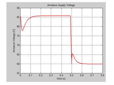
Figure 7: The input Voltage profile in SIMULINK for the DC Servomotor nominal model
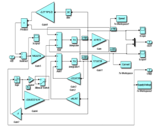
Figure 8: The detailed subsystem SIMULINK diagram of the DC servomotor nominal model
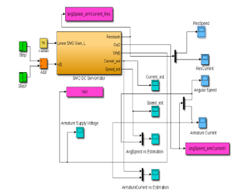
Figure 9: The overall SMO SIMULINK diagram of the DC servomotor model
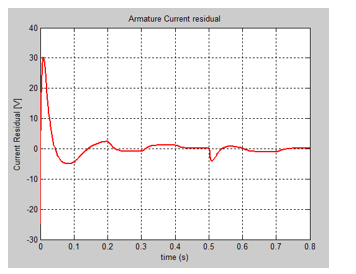
Figure 10: The SMO MATLAB simulations of armature current residual
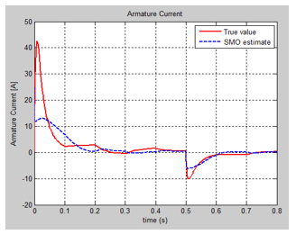
Figure 11: The SMO MATLAB simulations of armature current estimate versus true value
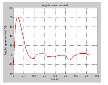
Figure 12: The SMO MATLAB simulations of angular speed residual
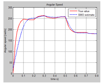
Figure 13: The SMO MATLAB simulations of angular speed estimate versus true value
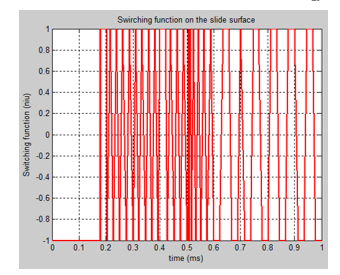
Figure 14: The SMO MATLAB simulations of SMO chattering evolution around the sliding surface
5. Fuzzy Sliding Mode Observer
5.1. The Dynamic Model of Fuzzy Sliding Mode Observer
In the most of practical situations the sliding mode systems experience several difficulties due to the chattering effects; therefore this inconvenient represents one of their main drawbacks [18]. The chattering phenomenon is well visible in Figure 14 that is undesirable because it involves high control activity and furthermore may excite high frequency unmodeled dynamics. The chattering effects induced by SMO estimator design with a high impact on the overall dynamics of the control system may be attenuated using different improvements into the original observer design.
The second method that is a fuzzy SMO approach is mentioned also in [18]. The basic idea is a new interpretation of the chattering effects seen as free estimations that may be achieved using linguistic variables instead of fixed numerical values. Thus, to improve the performance of the standard SMO developed in previous section is required some knowledge provided by an expert, so a new design approach known as Fuzzy logic SMO is developed [18]. The new intelligent FSMO estimation approach has the capability to maintain the robustness property of the clean standard SMO while the chattering phenomenon is significantly decreased. The dynamics of the fuzzy sliding mode observer is described by a similar equation (16) with slight changes by replacing the sign term by a linguistic variable, so a fuzzy term [18]:![]()
where the crisp output of the FSMO, is computed through the designed if – then rule-base considering the tracking errors: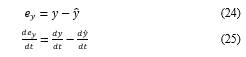
as input variables for fuzzy inference system (FIS) [18].
Compared to KF-SMO estimator the term of the observer (16) is replaced by a fuzzy output variable of the FIS to construct the fuzzy estimator FSMO (23). The hybrid structure of the SMO and FSMO estimators is build in SIMULINK and shown in Figure 15, with the main blocks detailed in the Figure 16 to Figure 19. Since the if-then rules of the fuzzy system are generated according to the properties of sign term, the FSMO is expected to be a robust observer [18]-[19]. The fuzzy if-then rules perform a nonlinear mapping from the input linguistic variables and to the output linguistic variable, as:![]()
5.2. Fuzzy Logic and Inference System Description Block
Fuzzy Logic (FL) is a computational paradigm that is based on the expert knowledge. Fuzzy Logic looks at the world in vague terms, almost in the same way that our brain takes in information (e.g. pressure is high, speed is slow, concentration is small, temperature is freezing), then responds with precise actions [19]. According to the same reference document… “the human brain can reason with uncertainties, vagueness, and judgments, and the computers can only manipulate precise valuations; therefore, fuzzy logic is an attempt to combine these two techniques”. Closing, unlike the false perception that “fuzzy” is a misnomer that has resulted in the mistaken suspicion that fuzzy logic is somehow less exacting than traditional logic however the practice reality has proved that the FL is in fact, a precise problem-solving methodology [19]. It is able also to simultaneously handle numerical data and linguistic knowledge. Fuzzy logic is a technique that facilitates the control of a complicated system without knowledge of its mathematical description, making the development and implementation of the control systems much simpler [19]. It requires no complicated mathematical models, only a practical understanding of the overall system behavior.
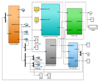
Figure 15: The SIMULINK hybrid structure of SMO and FSMO estimators’ models
Fuzzy logic differs from classical logic where an object takes on a value of either zero or one. In fuzzy logic, a statement can assume any real value between 0 and 1, representing the degree to which an element belongs to a given set [19]. Fuzzy Logic mechanisms can also lead to higher accuracy and smoother control, dealing with degrees of truth and degrees of membership. Most things in nature cannot be characterized with simple or convenient shapes or distributions. Membership functions characterize the fuzziness in a fuzzy set, whether the elements in the set are discrete or continuous, in a graphical form for eventual use in the mathematical formalisms of fuzzy set theory [19]. They can be of different shapes such as triangular, trapezoidal, singleton, sigmoidal function, Gaussian distribution, Wavelet functions, etc. The detailed hybrid structure SMO and FSMO –Fuzzy SIMULINK Block model is shown in Figure 16, including the manual switch from one structure to another one, all other blocks remaining common for the both structures.
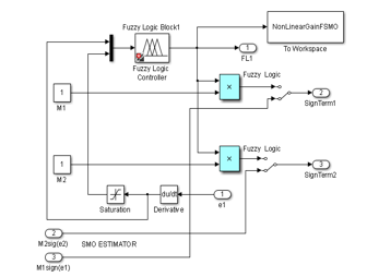
Figure 16: The SIMULINK hybrid structure SMO and FSMO –Fuzzy logic block model
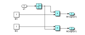
Figure 17: The SIMULINK hybrid structure SMO and FSMO –The gain matrix sign term Block
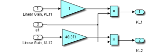
Figure 18: The SIMULINK hybrid structure SMO and FSMO –Linear gain matrix term block
In [18] to design the proposed FSMO estimator is chosen three membership functions of triangular shape corresponding to the input and output fuzzy sets of and as is shown in Figure 20. The linguistic labels used such as P, N, ZE, S, M and L stand for positive, negative, zero, small, medium and large, respectively. All seven possible combinations of two labels represent the input-output fuzzy set attached to each membership function and denote a negative-big, negative-small, negative-medium, zero, positive-small, positive-medium, and positive-big.
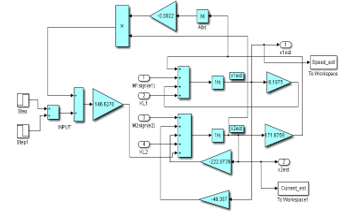
Figure 19: The SIMULINK hybrid structure SMO and FSMO –SMO Estimators Block
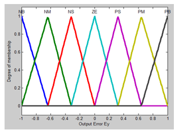
Figure 20: MATLAB Membership functions of input/output fuzzy sets e_y,(de_y)/dt and F_L [18]
Three main steps are involved to create a Fuzzy Inference System:
- Fuzzification that translates inputs into truth values
- Rule evaluation to compute output truth values
- Defuzzyfication that transfers truth values into output
In fuzzyfication step the inputs from a set of sensors (or features of those sensors) are mapped to values from 0 to 1 using a set of input membership functions, more precisely all the input variables are assigned degrees of membership in various classes [18]-[19]. In the rule evaluation step these inputs are applied to a set of if-then control rules. For example, to design the proposed FSMO estimator (23) a simple fuzzy rule Table 4 is constructed considering the following reaching and stability requirements [18]:
The output fuzzy set, is normalized in the interval [-1,+1], therefore:![]() Anytime when becomes a positive value, the membership function of is set in such a way that its sign becomes similar to that of and therefore While has a negative value, the reaching condition would be satisfied automatically. Therefore, for all the seven membership functions attached to each of two input variables of the fuzzy rule base, 49 if-then rules in Table 4 are obtained using an expert engineering knowledge in the electric drives machines field and satisfying the reaching conditions 1, 2 and 3. Fuzzy rules are always written in the following form: If (input1 is membership function1) and/or(input2 is membership function2) and/or …. Then (output is output membership function).Table 4: Rule bases of fuzzy logic sliding mode observer [7]
Anytime when becomes a positive value, the membership function of is set in such a way that its sign becomes similar to that of and therefore While has a negative value, the reaching condition would be satisfied automatically. Therefore, for all the seven membership functions attached to each of two input variables of the fuzzy rule base, 49 if-then rules in Table 4 are obtained using an expert engineering knowledge in the electric drives machines field and satisfying the reaching conditions 1, 2 and 3. Fuzzy rules are always written in the following form: If (input1 is membership function1) and/or(input2 is membership function2) and/or …. Then (output is output membership function).Table 4: Rule bases of fuzzy logic sliding mode observer [7]
| NB | NM | NS | ZE | PS | PM | PB | |
| NB | NB | NB | NB | NB | NM | NS | ZE |
| NM | NB | NB | NB | NM | NS | ZE | PS |
| NS | NB | NB | NM | NS | ZE | PS | PM |
| ZE | NB | NM | NS | ZE | PS | PM | PB |
| PS | NM | NS | ZE | PS | PM | PB | PB |
| PM | NS | ZE | PS | PM | PB | PB | PB |
| PB | ZE | PS | PM | PB | PB | PB | PB |
In many instances, it is desired to come up with a single crisp output from a FIS. This crisp number is obtained in a process known as defuzzification. In defuzzification step the fuzzy outputs are combined into discrete values needed to drive the control mechanism. There are two common techniques for defuzzifying:
- Center of mass – This technique takes the output distribution and finds its center of mass to come up with one crisp number, as is shown in [19].
- Mean of maximum – This technique takes the output distribution and finds its mean of maxima to come up with one crisp number, as is shown in [19].
More details about Laypunov’s stability and how to find an upper bound for the crisp value of output variable for the proposed FSMO (26) are given in [18].
5.3. Fuzzy Logic Sliding Mode Observer Simulation Results
We present in this section only the graphs with the evolution of the true values of the states and their FSMO estimated values, as well as the both residuals needed for developing the future fault detection and isolation strategies. The MATLAB simulations of armature current FSMO estimate versus the true values and its residual are shown in Figure 21 and Figure 24 respectively, and for angular speed in Figure 22 and Figure 23. During the simulations we didn’t find significant changes when we switch the gain matrix M values from and the simulation results remaining the same. For changes in the noise level from 0.1 spectral density powers to 10, so increased 100 times, we found also that FSMO is very accurate, so very robust to these changes, as we can see from the angular speed armature current residuals, as is shown in Figure 25 and Figure 26 respectively.
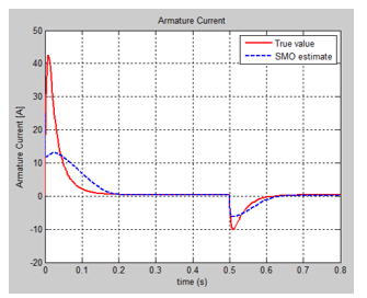
Figure 21: The SMOF simulations of MATLAB armature current estimation
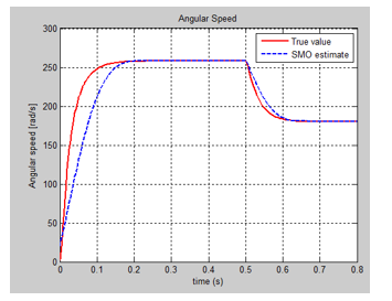
Figure 22: The SMOF simulations of MATLAB angular speed
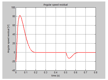
Figure 23: The SMOF MATLAB simulations of angular speed residual
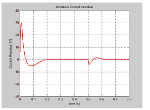
Figure 24: The SMOF MATLAB simulations of armature current residual
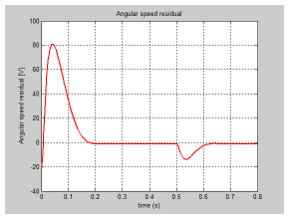
Figure 25: The SMOF MATLAB simulations of angular speed residual
Furthermore we tested the impact of changing the initial condition values of the estimated angular speed from 1 to -20 , and for armature current from 0 to -2.5 and we get the results shown in Figure 26 and Figure 27. We found also that FSOM algorithm is very robust to changes in the initial conditions values of the estimates.
Furthermore we tested also the accuracy of FSMO estimator for changes in the linear gain matrix coefficients from , as in all previous figures from this section, to that lead to the results shown in Figure 28 and Figure 29. These changes leads also to changes in the estimator dynamics, the poles of the estimators change the location , -222.8739 to another location given by , -222.8739. In the new location the FSMO estimator becomes more faster.
Closing, a high accuracy for FSMO estimator can be obtained by a suitable tuning of the gain matrices M and KL .
Compared the simulation results of the both estimators SMO and FSMO it is obviously that FSMO estimator performs better
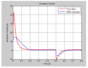
Figure 26: The SMOF simulations of MATLAB armature current estimation with new initial condition for estimated current (Robustness test)
All these results are encouraging for us to investigate a new approach to build more suitable fault detection and isolation control strategies in many control applications, using for estimation the developed hybrid structure with SMO and its improved version, a fuzzy sliding mode observer estimator (FSMO).
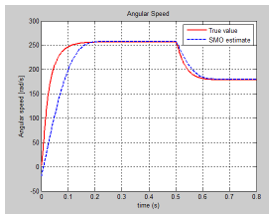
Figure 27: The SMOF simulations of MATLAB angular speed estimation with new initial condition for estimated current (Robustness test)
5.4. Summary of FSO Steps Design
To compute the output (26) of the FIS’ FSMO estimator given the inputs, one must go through six steps [19]:
Step1: Determining a set of fuzzy rules
Step2: Fuzzifying the inputs using the input membership functions
than SMO estimator in terms of accuracy and robustness, so FMSO is an improved version of SMO. This improvement is due to the fact that the chattering effects are reduced considerably, attenuating extremely the effect of the last term of (16),
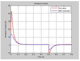
Figure 28: The SMOF simulations of MATLAB armature current estimation by changing the linear gain matrix coefficients (Robustness test)
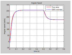
Figure 29: The SMOF simulations of MATLAB angular speed estimation by changing the linear gain matrix coefficients (Robustness test)
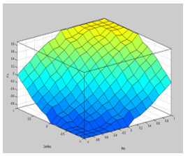
Figure 30: SIMULINK surface view of fuzzy sets e_y (Res),(de_y)/dt(DerRes) and F_L [18]
Step3: Combining the fuzzified inputs according to the fuzzy rules to establish rule strengthStep4: Finding the consequence of the rule by combining the rule strength and the output membership function (if it’s a Mamdani FIS),
Step5: Combining the consequences to get an output distribution, and
Step6: Defuzzifying the output distribution (this step applies only if a crisp output class) is needed), as is shown in Figure 30.
6. Conclusions
In this paper, we developed an improved version of a Sliding Mode Observer strategy design with a considerably changes of the approach followed in the conference paper [1] but using the same study case, namely a DC servomotor actuator with disturbance uncertainty that is integrated in the same control system structure. Encouraged by the results obtained in [1] we have investigated a new approach direction to improve the performance of the proposed SMO in terms of its accuracy, robustness and implementation design. The improved version of the SMO that we developed for the same single-input single-output control system is a fuzzy SMO estimator with a high estimation accuracy of the actuator states, and with a strong capability to attenuate the chattering effects of the sliding mode control design. It is also more robust to the changes in noise levels and in initial conditions values (guess values) of the estimates, and also to the input disturbance and modeling errors. In addition, its implementation design simplicity in real time recommends FSMO estimator without doubt as one of the most useful control strategy tool to be applied for our future developments in fault detection and isolation control applications. The design of new FDI control strategies will be an extension of our research in the future work based on the preliminary results obtained until now in real implementation and control design estimation techniques. Implementation in real time a Sliding Mode Observer for a linear DC Servomotor actuator with bounded disturbance uncertainty.
Conflict of Interest
The authors declare no conflict of interest.
- R-E. Tudoroiu, W. Kecs, Dobritoiu, N. Ilias, S.V. Casavela, N. Tudoroiu, “Real-Time Implementation of DC Servomotor Actuator with Unknown Uncertainty using a Sliding Mode Observer” in Proceedings of the Federated Conference on Computer Science and Information Systems, Gdansk, Poland, DOI: 10.15439/2016F95, ACSIS, ISSN 2300-5963, Vol. 8, pp. 841–848, 2015.
- E. Tudoroiu, A. Astilean, T. Letia, N. Iliasi, N.Tudoroiu, D. Burdescu, “Wireless UML-RT Simulator for Modeling and Implementing Dynamics Hybrid Structure of a Real Time PI DC Motor Control System”, The Journal of Economics and Technologies Knowledge , 1(4), 69-81, 2015.
- E. Tudoroiu, A. Astilean, T. Letia, V. Cretu, N. Iliasi, N. Tudoroiu, ”UML-RT Simulator for Modeling and Implementing Hybrid Structure Dynamics of a Real Time PID DC Servomotor Position Control System Strategy”, The Journal of Economics and Technologies Knowledge , 1(5), 68-77, 2015.
- R-E Tudoroiu, “Conceiving and Implementing Applications using Real-Time UML”, PhD Thesis, Cluj-Napoca Technical University, Romania, 2012.
- M. Galvez, “A New Fault Detection and Isolation Algorithm Applied to Dc Motor Parameters Supervision”, ABCM Symposium Series in Mechatronics , 5, 196-204, 2012, http://www.abcm.org.br/symposium-series/SSM_Vol5/Section_II_Control_Systems/07492.pdf
- Tudoroiu, K. Khorasani, “Satellite Fault Diagnosis using a Bank of Interacting Kalman Filters”, Journal of IEEE Transactions on Aerospace and Electronic Systems, DOI: 10.1109/TAES.2007.4441743, 43(4), 1334-1350, 2007.
- Isermann, Fault-Diagnosis Applications, Model-Based Condition Monitoring: Actuators, Drives, Machinery, Plants, Sensors, and Fault Tolerant Systems, DOI 10.1007/978-3-642-12767-0_3, Springer-Verlag Berlin Heidelberg, 2011.
- Haykin, Adaptive Filter Theory, 3rd ed., Prentice-Hall, Upper Saddle River, NJ., 1996
- L. Plett, G.L., “Extended Kalman filtering for battery management systems of LiPB-based HEV battery packs Part Background, Journal of Power Sources, ELSEVIER, 134, 252–261, 2004.
- I. Abbas, F.B. Hawraa, “Fault detection and isolation based on hybrid sliding mode observer and fuzzy logic”, Kufa Journal of Engineering, Iraq, ISSN 2207-5528, 6(1), 93-102, 2014.
- Alkaya, I. Eker, “Luenberger observer-based sensor fault detection: online application to DC motor”, Turkish Journal of Electrical Engineering and Computer Sciences, DOI: 10.3906/elk-1203-84, 22, 363-370, 2014.
- Chen, “Robust Fault Diagnosis and Compensation in Nonlinear Systems via Sliding Mode and Iterative Learning Observers”, PhD Thesis, Simon Frasier University, Canada, 2003.
- Loukil, M. Chtourou and T. Damak, “Synthesis of Nonlinear Observers for Actuator Fault Detection and Isolation”, International Journal of Computer Applications, 43(4), 27-32, 2012.
- K. Spurgeon, “Sliding Mode Observers – historical background and basic introduction”, Spring School, Aussois, 2015.
- K. Spurgeon, “Sliding Mode Observers – toward a constructive design framework”, Spring School, Aussois, 2015.
- G. Yan, C. Eduards, “Nonlinear robust fault reconstruction and estimation using a sliding mode observer”, Elsevier, ScienceDirect, Automatica, DOI:10.1016/j.automatica.2007.02.008, 43, 1605 – 1614, 2007.
- Castillo-Toledo, S. Di Gennaro, J. Anzurez-Marin, “On the fault diagnosis problem for non–linear systems: A fuzzy sliding–mode observer approach”, Journal of Intelligent and Fuzzy Systems, 20, DOI: 10.3233/IFS-2009-0427, IOS Press, 187–199, 2009.
- Keighobadi, P. Doostdar “Fuzzy Sliding Mode Observer for Vehicular Attitude Heading Reference System”, Journal of Scientific Research, Iran, DOI: 10.4236/pos.2013.43022, 4, 215-226, 2013, http://www.scirp.org/journal/pos
- Fuzzy Logic Tutorial, available online on the web site: http://www.massey.ac.nz/~nhreyes/MASSEY/159741/Lectures/Lec2012-3-159741-FuzzyLogic-v.2.pdf
- Control Tutorials for MATLAB, Carnegie Mellon Lab, University of Michigan, http://ctms.engin.umich.edu.