1. Introduction

Current 3D display systems include stereoscopy, integral photography, the differential binocular vision method, volumetric display, and holography [1]. With the rapid progress in image processing and stereoscopic technologies, three-dimensional (3D) images have become available not only on television but also in theaters, on game machines, and elsewhere. Unpleasant symptoms such as asthenopia, dizziness, and nausea have been observed in some individuals viewing 3D videos [2]. While the symptoms of general motion sickness include dizziness and vomiting, the phenomenon of visually-induced motion sickness (VIMS) is not fully understood. Currently, there is insufficient knowledge regarding the effects of stereoscopic images on the living body, and basic research is thus important [3].

Contradictory messages originating from different sensory systems, or the absence of a sensory message that is expected in a given situation, are thought to lead to a feeling of sickness. Spatial localization of self-becomes unstable and produces discomfort. Researchers agree that there is a close relationship between the vestibular and autonomic nervous systems both anatomically and electrophysiologically. Motion sickness is considered to be caused by excess signals from the vestibular nuclei to the hypothalamus. This strongly indicates that the equilibrium system is associated with the symptoms of motion sickness [4] and provides a basis for the quantitative evaluation of motion sickness based on body sway, an output of the equilibrium system.

Stabilometry is a useful test of body equilibrium for investigating the overall equilibrium function. Stabilometry methods are presented in the standards of the Japanese Society for Equilibrium Research and international standards [5]. Stabilometry is a simple test in which 60-second recording starts when body sway stabilizes [6]. Objective evaluation is possible by computer analysis of the speed and direction of the sway, enabling diagnosis of a patient’s condition [7].

In previous studies, subjective exacerbation and deterioration of equilibrium function were observed after peripheral viewing of a 3D video clip [8, 9]. A persistent influence has been observed while subjects view a poorly depicted background element peripherally, which generates depth perception that contradicts daily life. In this study, we examined the effect of viewing 3D video clips on equilibrium function systems using mathematical analysis.

2. Material and Method

Sixteen healthy male subjects (mean age ± standard deviation: 22.2 ± 0.7 years) participated voluntarily in the study. We ensured that the body sway was not affected by environmental conditions. We used an air conditioner to adjust the temperature to 25 °C in the exercise room. The experiment was explained to all subjects and written informed consent was obtained in advance.

Experiments were performed in a dark room to avoid irritation from sources other than the video. 2D or 3D video clips were shown on a 3D display (KDL 40HX80R; SONY) placed 2 meters away from the subject. In the video clip used in the experiment, a sphere moved around the screen (Figure 1). A comparison was then made with subjects who were asked to simply gaze at a point 2 meters in front of them at eye level where no video clips were displayed. The experiments were carried out in random order. Each experiment was carried out on a separate day.

The subjects stood without moving on the detection stand of a stabilometer (Wii Balance Board; Nintendo) in the Romberg posture with their feet together for 30 seconds before the sway was recorded. Each sway of the center of pressure (COP) was then recorded at a sampling frequency of 20 Hz during the measurement; subjects were instructed to maintain the Romberg posture for the 60 seconds. The x–y coordinates were recorded with subjects’ eyes open for each sampling time, and stabilograms were constructed from the time sequences. The following quantitative indices were calculated:

• Area of sway: Area of a region surrounded (enveloped) by the circumferential line of sway on the x–y coordinates. An increase in the value represents a more unstable sway;
• Total locus length: Total extended distance of movement of the COP within the measurement time period. An increase in the value represents a more unstable sway;

The area of sway and total locus length are analytical indices of stabilograms that were used in previous studies. We used these based on the definitions established by the Japanese Society for Equilibrium Research.

Figure 1: The video clip shown to the subjects on a 3D display.

3. Mathematical Models of Body Sway

In stabilograms, variables x (right designated as positive) and y (anterior designated as positive) are regarded to be independent [10]. A linear stochastic differential equation (Brownian motion process) has been proposed as a mathematical model to describe body sway [11, 12, 13]. To describe the individual body sway, we show that it is necessary to extend the following nonlinear stochastic differential equations: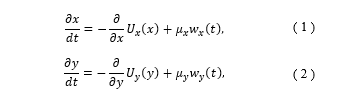

where  and  are pseudorandom numbers produced by white Gaussian noise [14]. The following formulas describes the relationship between the distribution in each direction,  and  and the temporal averaged potential constituting the stochastic differential equations (SDEs):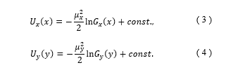

The variance of stabilograms depends on the temporal averaged potential function (TAPF) with several minimum values when it follows the Markov process without abnormal dispersion. SDEs can represent movements within local stability with a high-frequency component near the minimal potential surface, where a high density at the measurement point is expected.

4. Numerical Analysis

A histogram of each stabilogram was obtained. The mean of each stabilogram was set to be (0, 0) by statistical processing. We compared histograms that were composed of all subjects’ stabilograms with eyes open. The TAPFs while viewing 2D and 3D video clips were determined from the histograms using Eq. (5, 6). The TAPFs were regressed by the following degree 4 polynomial (Figures 2).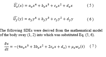

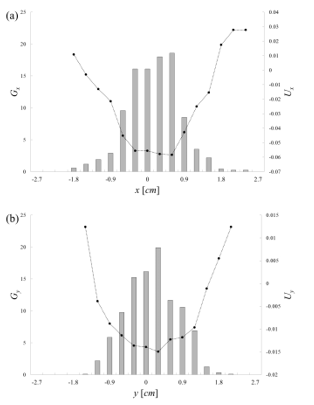
Figure 2: A typical example of TAPF derived from stabilograms during exposure to the 3D video clip: x direction (a), y direction (b).

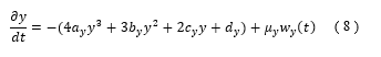
Here, the constants  and represent the noise amplitudes. We rewrote Eq. (7, 8) into a difference equation and obtained numerical solutions with the Runge-Kutta-Gill formula as the numerical calculus.

In Eq. (7, 8), the initial values of (x, y) were set to be (0, 0). Pseudorandom numbers (mean ± standard deviation: 1 ± 1) were generated to substitute for white Gaussian noise . The noise amplitude  and time step Δt were set to be 0.1, 0.2, …, 4.0 and 0.001, 0.002, …, 0.05, respectively. Numerical analysis was employed for 11,200 steps, and the first 10,000 steps of the numerical solutions were discarded due to dependence of the initial value. The area of sway ( ) and the total locus length ( ) were also calculated in these numerical solutions. Designating the measured the area of sway and the total locus length as ( ) and ( ), errors (E) between the numerical solutions of the mathematical model and measured data were defined as follows: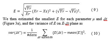

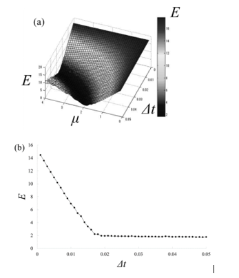
Figure 3: A typical evaluation, E, for numerical solutions to the mathematical model for Control with the following parameters: (μ, Δt) (a), Δt (b).

was calculated to determine the plateau of the error E. The left bound Δt* was defined as the optimum value for the plateau in the case that the variance (10) exceeded 0.3 in this study (Figure 3b). This parameter was calculated for each subject.

5. Result

Stabilograms measured during exposure to a 2D video clip were compared with those of a 3D video clip (Figures 4). We also calculated the area of sway and the total locus length for each stabilogram (Figures 5). These were compared by Wilcoxon signed-rank test with each index for the stabilometry. The significance level was set to be 0.10. The results of the Wilcoxon signed-rank test showed that the value of the total locus length while viewing the 3D video clip was significantly smaller than that while viewing the 2D video clip (p<0.10).

Histograms of each component were obtained from subjects’ stabilograms in each condition. The TAPFs were constructed from the histograms using Eqs. (5, 6). The TAPFs were sufficiently regressed by polynomials of degree four. Eqs. (7, 8) were rewritten into difference equations, and the numerical solutions were obtained with the Runge-Kutta-Gill formula (Figures 6). The area of sway and total locus length were also calculated in these numerical solutions. The smaller the E, the better the description the numerical simulation could give (Figures 7). The value of errors E was evaluated with the control parameters Δt and μ in the abovementioned difference equations (Figures 8). The smallest Δt was obtained while viewing the 3D video clip (p<0.10) (Figure 8b). The largest μ was obtained while

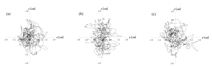
Figure 4: Typical stabilograms obtained from a subject: Control (a); the 2D (b); the 3D (c).

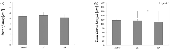
Figure 5: Results of sway values (average ± SE): the area of sway (a); the total locus length (b).

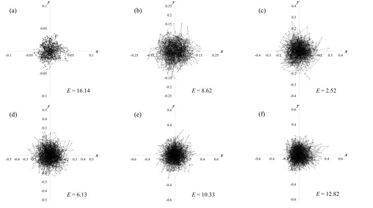
Figure 6: Typical examples of numerical solutions at μ = 3.9 and the following time step:
Δt = 0.001 (a); Δt = 0.01 (b); Δt = 0.02 (c); Δt = 0.03 (d); Δt = 0.04 (e); Δt = 0.05 (f).

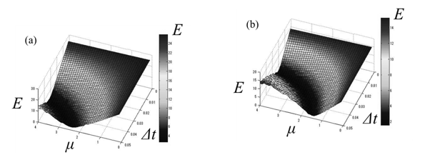
Figure 7: A typical evaluation for numerical solutions to the mathematical model while viewing the video clip: the 2D (a); the 3D (b).

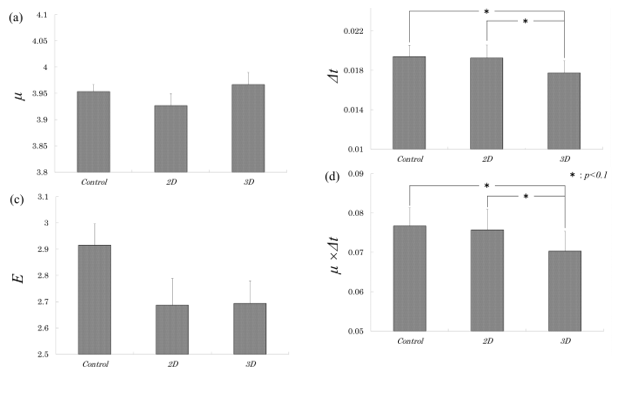
Figure 8: Results of optimum value (average ± SE): μ (a); Δt (b); E (c); μ × Δt (d).

viewing the 3D video clip, and the smallest one was obtained while viewing the 2D video clip (Figure 8a). In this paper, μ × Δt was evaluated for rigidity in the postural control. As shown in Figure 8d, the value of μ × Δt while viewing the 3D video clip was smaller than in the other cases (p<0.10).

6. Discussion

Previously, we evaluated body sway by conducting stabilometry studies with simple use of the analytical indices for stabilograms. In this study, we further obtained TAPFs in the SDEs as mathematical models of body sway. We also examined whether there is any remarkable evolution in the potential functions to control standing posture during exposure to stereoscopic video clips.

The previous research showed that the sway values after viewing a 3D video clip are larger than those in other conditions, including after viewing the 2D. However, as a result of the Wilcoxon signed-rank test in this study, the value of the total locus length while viewing the 3D video clip was found to be significantly smaller than that while viewing the 2D video clip (p<0.10). Therefore, we proposed the mathematical model while viewing the video clips and evaluated the stabilograms by numerical analysis. In the numerical solution, the area of sway and the total locus length were proportional to the product μ × Δt. In this study, the results when Δt was around 0.019 and μ was around 3.9 showed values close to the sway values in the measurements, such as the area of sway and the total locus length.

A flexible system to control body sway reduces the product of μ × Δt. Fine postural control, which has been regarded as an anomalous system to control the upright posture, might be seen before the outbreak of motion sickness. This anomalous process is considered to be a clue to elucidating the procedure of the motion sickness and predicting the time when the first symptom of motion sickness will appear. In the next step, we will extend the viewing time of the video and use a subjective questionnaire to examine the relationship between the VIMS and body sway.

We have also succeeded in showing that postural control can be evaluated by numerical analysis with our mathematical model in the case that differences cannot be seen in the stabilograms with use of previous indices such as the area of sway and total locus length. Using a mathematical model for the evaluation of the stabilograms may contribute to the elucidation of the postural control system.

7. Conclusion

Previously, we evaluated body sway by conducting stabilometry studies with simple use of the analytical indices for stabilograms. In this study, we obtained TAPFs in the SDEs as mathematical models of body sway. We also examined whether there is any remarkable evolution in the potential functions to control the standing posture during the exposure to stereoscopic video clips. As a result, we verified that 3D viewing effects on our equilibrium function can be seen with the use of a mathematical model.

Conflict of Interest

The authors declare no conflict of interest.

Acknowledgment

This work was supported in part by the Japan Society for the Promotion of Science, Grant-in-Aid for Scientific Research (B) Number 24300046 and (C) Number 26350004.

1. Gabor, “A New Microscopic Principle,” Nature, 161, 777–779, 1948.
2. International standard organization, “IWA3: 2005 Image Safety-Reducing Determinism in a Time Series,” Phys. Rev. Lett., 70, 530–582, 1993.
3. Sumio, I. Shinji, “Visual Comfort and Fatigue Based on Accommodation Response for Stereoscopic Image,” The Institute of Image Information and Television Engineers, 55 (5), 711–717, 2001.
4. H. Barmack, “Central Vestibular System: Vestibular Nuclei and Posterior Cerebellum,” Brain Res. Bull., 60, 511–541, 2003.
5. Japan Society for Equilibrium Research, “Standard of Stabilometry,” Equilib. Res., 42, 367–369, 1983.
6. S. Kaptyen, W. Bles, C.J. Njiokiktjien, L. Kodde, C.H. Massen, J.M. Mol, “Standarization in Platform Stabilometry being a part of Posturography,” Agreessologie, 24, 321–326, 1983.
7. Hase, Y. Ohta, “Meaning of Barycentric Position and Measurement Method,” J. of Environ. Eng., 8, 220–221, 2006.
8. Yoshikawa, F. Kinoshita, K. Miyashita, A. Sugiura, T. Kojima, H. Takada, M. Miyao, “Effects of Two-Minute Stereoscopic Viewing on Human Balance Function,” In: Antona, M., Stephanidis C. (eds.) UAHCI/HCII 2015 Part II. LNCS, 9176, 297–304, 2015.
9. Takada, Y. Fukui, Y. Matsuura, M. Sato, H. Takada, “Peripheral Viewing during Exposure to a 2D/3D Video Clip: Effects on the Human Body,” Environ Health Prev Med., 20, 79-89, 2015.
10. A. Goldie, T.M. Bach, O.M. Evans, “Force Platform Measures for Evaluating Postural Control: Reliability and Validity,” Arch. Phys. Med. Rehabil., 70, 510–517. 1986.
11. E.A. Emmerrik, R.L.V. Sprague, K.M. Newell, “Assessment of Sway Dynamics in Tardive Dyskinesia and Developmental Disability,” Sway Profile Orientation and Stereotypy. Moving Dis., 8, 305-314, 1993.
12. J. Collins, C.J.D. Luca, “Open Loop and Closed-Loop Control of Posture: A Random-Walk Analysis of Center of Pressure Trajectories,” Exp. Brain Res., 95, 308–318, 1993.
13. K. M. Newell, S.M. Slobounov, E.S. Slobounova, P.C. Molenaar, “Stochastic Processes in Postural Center of Pressure Profiles,” Exp. Brain Res., 113, 158–164, 1997.
14. H. Takada, Y. Kitaoka, Y. Shimizu, “Mathematical Index and Model in Stabilometry,” Forma, 16, 17–46, 2001.

(Click to view)

(Click to view)