Numerical Analysis of Drawdown in an Unconfined Aquifer due to Pumping Well by SIGMA/W and SEEP/W Simulations
Numerical Analysis of Drawdown in an Unconfined Aquifer due to Pumping Well by SIGMA/W and SEEP/W Simulations
Volume 1, Issue 1, Page No 11-18, 2016
Author’s: Imran Arshada) 1, Muhammed Muneer Babar2, Natasha Javed3
View Affiliations
1Agriculture Engineer, Star Services LLC, Al Muroor Road – Western Region of Abu Dhabi, United Arab Emirates (UAE).
2Professor, IWREM – CASW, MUET, Jamshoro, Pakistan,
3Ph.D Student (Applied Hydrology), CEES, University of the Punjab, Lahore, Pakistan.
a)Author to whom correspondence should be addressed. E-mail: engr_imran1985@yahoo.com
Adv. Sci. Technol. Eng. Syst. J. 1(1), 11-18 (2016); ![]() DOI: 10.25046/aj010102
DOI: 10.25046/aj010102
Keywords: Finite Element Modeling Pumping Well, Observation Well, SEEP/W, SIGMA/W, Drawdown, Unconfined Aquifer

Export Citations
In the present study a computer model of a pumping well has been developed and calibrated by using two slave programs of Geo-Slope software, i.e. (SIGMA/W and SEEP/W). The model has been used to study the behaviour of watertable and drawdown in an aquifer during pumping. SIGMA/W program was used to compute initial pore-pressure within an aquifer, while SEEP/W program was used to analyze the change in pore-pressure and drawdown during pumping respectively. From the results it is revealed that the vectors displaying the movement of the flow direction towards discharge well due to which decline in watertable occurs and a cone of depression and drawdown curve was formed. Comparison of the experimental and simulated data showed a good agreement among them. The drawdown line has been simulated for each concern depth and at each interval of time, which was further compared with the actual data for the computation of model efficiency. The performance of the model was evaluated on the basis of statistical parameters, i.e. mean error, root mean square error and model efficiency; these results are presented in Table 7. Statistical analysis of all the research data, i.e. RMSE, ME, R.E, and EF was found to be 0.134 m and 0.126 m, 3.05% and 98.86% respectively. Additionally verifiability of the model was also made by comparing observed and simulated values of observation wells (piezometeric heads); such graph is illustrated in Figure 5. The slope of the line was observed to be approximately at 45 degrees; thus the figure indicates no considerable difference between observed and simulated head values for all the observation wells. Consequently, it is concluded that simulated values of piezometeric heads are not much different than the observed ones. The results support the use of SIGMA/W and SEEP/W programs as a tool for investigating and designing pumping well practices.
Received: 30 March, 2016, Accepted: 23 April 2016, Published Online: 25 April 2016
Acknowledgement
The authors wish to express their gratitude to WAPDA Hyderabad – Pakistan, representatives for their kind cooperation throughout the research study and all other individuals who have been source of help throughout the research period.
1. Introduction
Large parts of the arid areas of Pakistan depend on canal and groundwater. Groundwater is used for drinking and domestic purposes meeting irrigation need, including livestock requirement and in industries. Groundwater also contributes to the environmental flows [1]. Understanding groundwater resources are important in developing responses to various groundwater problems such as groundwater depletion, and groundwater pollution. Groundwater basically occurs in aquifers in the pore spaces of fractures and other such opening in the rocks. Aquifers are saturated rocks or materials derived from rocks like sand and gravel capable of storing and transmitting water underneath the earth’s surface [2]. Aquifers provide water to wells from there it can be pumped out. Open wells, bore wells and tubewells are man-made mechanisms used to extract a groundwater[3]. Aquifers also fed streams and rivers, especially during the dry season. Stream flows fed by groundwater are called as base flows. Aquifers may occur at relatively shallow depth below the ground surface and groundwater in such aquifers can be set to be at atmospheric pressure, such aquifers are called as unconfined aquifers.
Sometimes, aquifer occurs at much greater depth below the ground. Groundwater contained in such aquifers is at a pressure exceeding atmospheric pressure due to overlie and underlie rocks. Such aquifers are called as confined aquifers. The type of rock, its structure and especially the openings within decides how much water the rock will store and how quickly it will allow it to flow from one point to another within the aquifer. Pumping of groundwater from wells and the discharge to base flow cause aquifers to deplete [4]. Aquifers may sufficiently fill up again if wells have to sustain pumping for many years and streams must remain alive longer. This refilling of aquifer is called as groundwater recharge. Hydro-geological investigations are important in understanding the problems of groundwater over exploitation, quality, recharge and reuse.
Pumping tests provide the information regarding the storage and transmission properties of aquifers. These tests also indicate the capacity of a well to yield water. During the pumping test a well is pumped and water levels are measured in the pumping well as well as in specially made adjacent bore holes. The drop in water levels in an aquifer observed in these wells during pumping is called drawdown. The water level in a well fluctuates during drawdown and recovery is a response to the pumping in the well. Nowadays, many computer software’s has come into general use, and any hard computations and simulation can be carried out through them by giving them appropriate inputs and data [5]. This results in less error frequency and more detailed analysis when compared with field observations. In order to simulate the water fluctuation process due to pumping through different soils regimes there are many numerical solution methods, i.e. Finite Differences (FDM), Finite Elements (FEM) and Boundary Elements (BEM) [6]. But the FEM is an effective numerical technique because of its numerous applied fields such as groundwater flow, multiphase flow, and mass flow through pours medium. The primary focus of this research work is to study the water level behavior in an unconfined aquifer due to groundwater movement caused by pumping through two slave programs of Geo-Slope i.e. SEEP/W and SIGMA/W for the development of numerical models and its analysis.
2. Objectives
The objectives of this research work were to compare the SIGMA/W and SEEP/W simulations of pore-pressure change in an unconfined aquifer caused by pumping with field observations, to compute the flow vectors, to analyze the movement of groundwater movement, and to simulate the drawdown curve for different time intervals.
3. Materials and Methods
3.1. Location
The study was undertaken in an area of Tando Soomro, which is 50 km away from Hyderabad, Sindh – Pakistan and containing homogeneous and anisotropic type unconfined aquifer located over an impervious layer in the year 2011-2012. The area receives irrigation water supplies through the canal system and also supplemented by groundwater supplies. The area has a number of fresh water tubewells meant for supplementing irrigation water requirement during surface water deficiency. The soil of the study area was mostly sandy loamy clayey up to 8 m depth, average ground surface level (elevation) with respect to MSL (Mean Sea Level) was 16m and watertable was around 3.77 m deep from the ground surface.
3.2. Field Experiment
In order to achieve the objective of the present research work a five year old data were depicted in this research. A field experiment was conducted by WAPDA during the year 2011 – 2012 to analyze the watertable behavior through the sandy loamy clayey soil. The experiment was conducted on a WAPDA installed tube-well (discharge well) along with 5 bore holes at a distance of 900 m, 1,800 m, 3,000 m, 4,800 m, and 5,100 m respectively. Before commencing the test, in preliminary step static water level within the pumping well and in all bore holes was recorded. The static water level is the non-pumping water level within the discharge well and borehole without the influence of pumping. After taking all the preliminary data before pumping the pump was then started and data collected at different intervals of time for discharge well and bore holes. As the study was conducted on constant discharge therefore, with the help of pump / valve discharge rates were kept as constant as possible throughout the research work till the pumping stopped. Finally, on the basis of results obtained from the experiment, it was utilized in developing numerical modeling and computations for different parameters were took place accordingly.
3.3. Steps for Modeling
In order to develop a 2- D finite element model, two slave programs of Geo-Slope Software i.e. (SEEP/W) for the flow analysis and (SIGMA/W) for the volume change analysis within the aquifer was used. A powerful and flexible feature in SIGMA/W has an ability to compute the volume change arising from an independently computed change in pore-pressure. Initially, by using SIGMA/W Insitu analysis a 2-D finite element mesh was generated to obtain the initial pore-pressure within the aquifer. The dimensions of the mesh were used for both SIGMA/W and SEEP/W programs to simulate the studied cases. The mesh is around 10,800 m long and 16 m in depth. The average ground elevation was 16m and the difference between the elevation of static watertable and ground surface was 3.77 m respectively. The domain is discretized into a mesh by 396 elements through placement of nodal points 479. The partially penetrating pumping well was then centrally assigned at a distance 5,400 m along with five adjacent bore holes on left and right side of the pumping well at a distance of 900 m, 1,800 m, 3,000 m, 4,800 m, and 5,100 m respectively. After the development of numerical model, the material properties for the materials used in subject mesh were calibrated. After calibration, it is then verified by the SIGMA/W software and computation for initial change in pore-pressure is carried out accordingly.
After the computation of initial pore-pressure within the aquifer the model was then imported to the SEEP/W program to find out the change in pore-pressure at different depths respectively. To solve the model numerically, initial and boundary conditions are specified first. In the present case, Neumann type boundary with the zero flux condition is executed on bottom, left and right of the mesh. Furthermore, Dirichlet boundary condition are assigned to the top of bore holes, while rest of the boundary nodes are treated as Neumann nodes with zero flux condition in such a way that the water level within the aquifer must remain at the initial watertable. After assigning the boundary nodes material properties for the materials used in subject mesh were calibrated and assigned accordingly.
With the objective to get precise results it has been assumed that the pumping will be controlled, so that the water level in the well will not drop below the top of the screen. H-type boundary condition i.e. (zero pressure) was then applied at the top of the well screen and which will increase hydrostatically with the depth within the well screen. Now as the starting and final pore-pressure conditions are known, therefore in order to find out the drawdown within the aquifer initial boundary conditions are required therefore, on the basis of experimental data the known boundary conditions was assigned to the pumping well for different interval of time accordingly. The time step sequence consists of 24 steps. Time starts by Zero minute and ends by 240 minutes for different depths in pumping well the drawdown in observation wells (bore holes) were recorded accordingly. Finally simulated results obtained from the SEEP/W and SIGMA/W program for each depth are compared with the observed data obtained from the experiment accordingly.
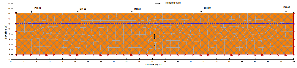
Figure 1: The mesh of the domain showing the boundary conditions for SIGMA/W analysis
4. Results and Discussion
4.1. FEM Mesh Formation and Its Verification
The FEM mesh for the selected case is composed of four types of elements, i.e. triangular, square, rectangular and trapezoidal type of elements of 3 ft size (Figure 1). The domain is discretized into a mesh by 396 elements through placement of nodal point’s 479. The material properties for subject mesh with proper dimensions are made as input to the SIGMA/W program and verification has been made accordingly. As the soil was mostly sandy loamy clay up to 8 m depth from the ground surface therefore, it is assumed that the complete soil region of the subject is to be considered as sandy loamy clay. The saturated hydraulic conductivities kx- and ky- are worked out as 3.455 x 10⁻⁴ m/s and 3.455 x 10⁻⁴ m/s, and the constant pumping rate of 0.042 m3/sec was adopted for the given aquifer. After assigning materials the initial watertable at 3.77 m from the ground surface was assigned accordingly. After all the necessary inputs, the computer program SIGMA/W verified the mesh development and delivered report that the vertical and horizontal meshing is strong enough and there is no error in formation of mesh model. Thus the model is ready for computation and analysis of the results.
Likewise, SEEP/W program is used to find out the change in pore-pressure at different depths respectively for the present case (Figure 2). According to the given conditions the Neumann type boundary with zero flux condition is executed on bottom, left and right of the mesh and Dirichlet boundary condition are assigned on the top of bore holes, while rest of the boundary nodes are treated as Neumann nodes with zero flux condition respectively. Then geological parameters and material properties are then calibrated accordingly. After all the necessary inputs, the computer program SEEP/W verified the mesh development and delivered report there is no error in formation of numerical model. Thus the model is ready for computation and analysis of the results.
4.2. Analysis of Initial Pore-Pressure by SIGMA/W
In order to solve the numerical model the initial pore-pressure conditions are required so that we can obtain the correct change in pore-pressures. Therefore, to study the behavior of drawdown in an aquifer due to pumping initially, SIGMA/W program was used to acquire the initial pore-pressure within the aquifer for (t = 0 minutes) Figure 3. The initial pore pressure computed from SIGMA/W was then used by SEEP/W to find out the change in pore-pressure at different depths respectively.
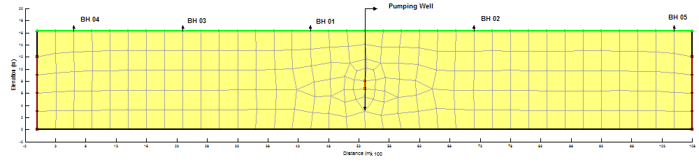
Figure 2: The mesh of the domain showing the boundary conditions for SEEP/W analysis

Figure 3: Initial Pore-Pressure within the Aquifer For (t = 0 minutes) by SIGMA/W
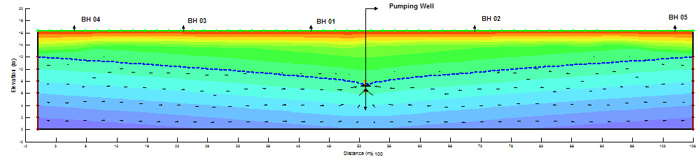
Figure 4.1: Drawdown at (t = 10 minutes) by SEEP/W Program.
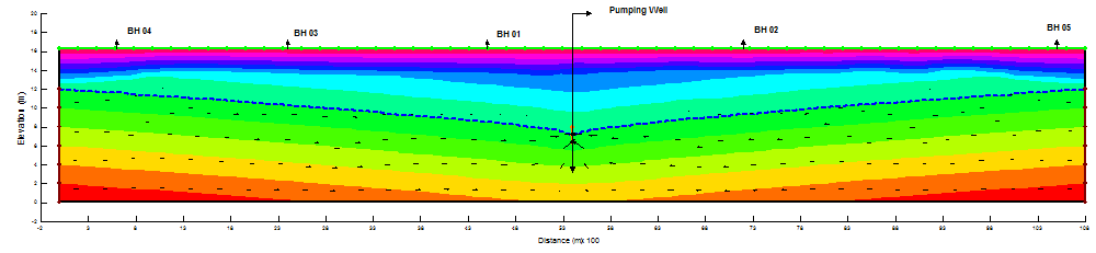
Figure 4.2: Drawdown at (t = 25 minutes) by SEEP/W Program.
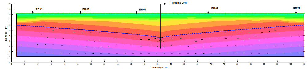
Figure 4.3: Drawdown at (t = 75 minutes) by SEEP/W Program.
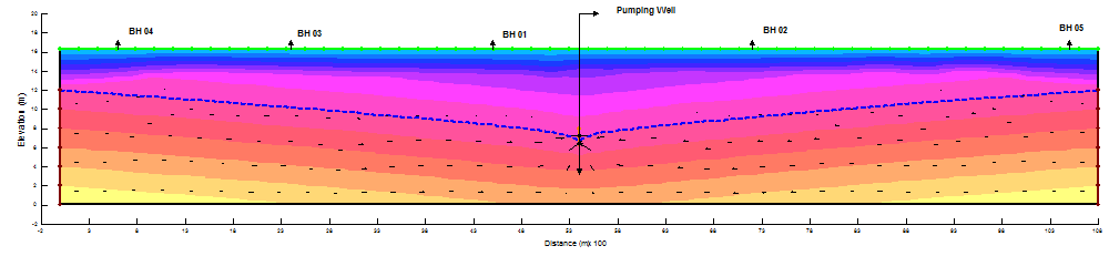
Figure 4.4: Drawdown at (t = 120 minutes) by SEEP/W Program.
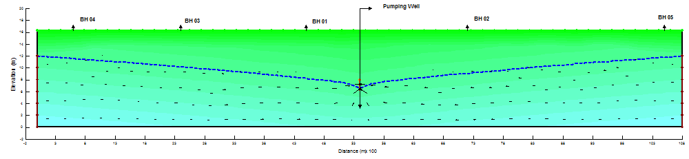
Figure 4.5: Drawdown at (t = 180 minutes) by SEEP/W Program.
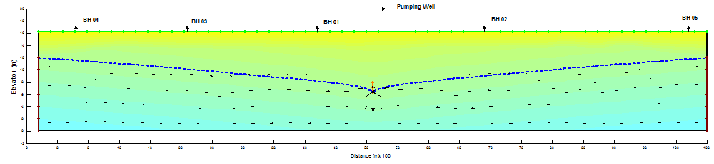
Figure 4.6: Drawdown at (t = 240 minutes) by SEEP/W Program.
4.3. Analysis of Change in Pore-Pressure at Different Depths by SEEP/W
The effect of the pumping is analyzed using a steady-state SEEP/W analysis. Boundary conditions are applied on the left and right ends, so that the water level remains at the initial watertable. Now as the initial and final pore-pressure conditions are known, the computation of drawdown in all five observation wells and analysis of the behavior of aquifer during pumping was conducted accordingly. The resulting long-term (steady-state) pore-pressure conditions are shown in Figure 4.1 – Figure 4.6.
Table 1. Observed Piezometeric Heads for Pumping Well Under Steady- State Conditions for an Unconfined Aquifer.
| Date and Time | Elapsed Time | Elevation | Meter to Water | Drawdown Ho | Remarks | |
| Min | Meter | Ho | Do | |||
| 9:00 AM | 12.23 | 3.77 | 0 | Non-Pumping Level | ||
| 9:15 AM | 0 | 12.23 | 3.77 | 0 | Pumping Started | |
| 9:17 AM | 2 | 7.8 | 8.2 | 4.43 | ||
| 9:19 AM | 4 | 7.74 | 8.26 | 4.49 | ||
| 9:21 AM | 6 | 7.65 | 8.35 | 4.58 | ||
| 9:23 AM | 8 | 7.56 | 8.44 | 4.67 | ||
| 10:00 AM | 45 | 7.1 | 8.9 | 5.13 | ||
| 10:15 AM | 60 | 7.07 | 8.93 | 5.16 | ||
| 10:30 AM | 75 | 7.04 | 8.96 | 5.19 | ||
| 10:45 AM | 90 | 7.01 | 8.99 | 5.22 | ||
| 11:00 AM | 105 | 6.85 | 9.15 | 5.38 | ||
| 11:15 AM | 120 | 6.82 | 9.18 | 5.41 | ||
| 11:30 AM | 135 | 6.79 | 9.21 | 5.44 | ||
| 11:45 AM | 150 | 6.76 | 9.24 | 5.47 | ||
| 12:00 PM | 165 | 6.73 | 9.27 | 5.5 | Afternoon | |
| 12:15 PM | 180 | 6.64 | 9.36 | 5.59 | ||
| 12:30 PM | 195 | 6.61 | 9.39 | 5.62 | ||
| 1:15 PM | 240 | 6.52 | 9.48 | 5.71 | Pumping Stopped |
From Figures it is revealed that the water flow vectors are moving towards the pumping well due to which decline in watertable occurs and a cone of depression and drawdown curve was formed. The complete summary of results are elaborated in Table 1 – Table 6 respectively.
Table 2. Observed and Simulated piezometeric heads for Observation Well 01 under steady- state conditions at different interval of time.
| Elapsed Time Min. | Meter to Water | Meter to Water | Drawdown | Drawdown | Remarks | |
| Min. | Ho | Hs | Do | Ds | ||
| 3.77 | Non-Pumping Level | |||||
| 0 | 3.77 | Started Pumping | ||||
| 2 | 6.68 | 6.83738 | 2.91 | 2.97856 | ||
| 4 | 6.74 | 6.82625 | 2.97 | 3.00856 | ||
| 6 | 6.83 | 6.99341 | 3.06 | 3.13459 | ||
| 8 | 6.92 | 7.13037 | 3.15 | 3.24795 | ||
| 45 | 7.38 | 7.55512 | 3.61 | 3.6963 | ||
| 60 | 7.41 | 7.58633 | 3.64 | 3.72751 | ||
| 75 | 7.44 | 7.61753 | 3.67 | 3.75871 | ||
| 90 | 7.47 | 7.64874 | 3.7 | 3.78992 | ||
| 105 | 7.63 | 7.80477 | 3.86 | 3.94595 | ||
| 120 | 7.66 | 7.83621 | 3.89 | 3.97727 | ||
| 135 | 7.69 | 7.80669 | 3.92 | 3.97754 | ||
| 150 | 7.72 | 7.89908 | 3.95 | 4.03992 | ||
| 165 | 7.75 | 7.91395 | 3.98 | 4.06274 | Afternoon | |
| 180 | 7.84 | 7.9957 | 4.07 | 4.15011 | ||
| 195 | 7.87 | 7.9943 | 4.1 | 4.16428 | ||
| 240 | 7.96 | 8.14804 | 4.19 | 4.28922 | Started Stopped |
Table 3. Observed and Simulated piezometeric heads for Observation Well 02 under steady- state conditions at different interval of time.
| Elapsed Time Min. | Meter to Water | Meter to Water | Drawdown | Drawdown | Remarks | |
| Min. | Ho | Hs | Do | Ds | ||
| 3.77 | Non-Pumping Level | |||||
| 0 | 3.77 | Started Pumping | ||||
| 2 | 6.2 | 6.34607 | 2.43 | 2.48725 | ||
| 4 | 6.26 | 6.34018 | 2.49 | 2.52249 | ||
| 6 | 6.35 | 6.5021 | 2.58 | 2.64328 | ||
| 8 | 6.44 | 6.63606 | 2.67 | 2.75364 | ||
| 45 | 6.9 | 7.06381 | 3.13 | 3.20499 | ||
| 60 | 6.93 | 7.09502 | 3.16 | 3.2362 | ||
| 75 | 6.96 | 7.12622 | 3.19 | 3.2674 | ||
| 90 | 6.99 | 7.15743 | 3.22 | 3.29861 | ||
| 105 | 7.15 | 7.31346 | 3.38 | 3.45464 | ||
| 120 | 7.18 | 7.34488 | 3.41 | 3.48595 | ||
| 135 | 7.21 | 7.31916 | 3.44 | 3.49001 | ||
| 150 | 7.24 | 7.40773 | 3.47 | 3.54857 | ||
| 165 | 7.27 | 7.42361 | 3.5 | 3.5724 | Afternoon | |
| 180 | 7.36 | 7.50608 | 3.59 | 3.66049 | ||
| 195 | 7.39 | 7.50666 | 3.62 | 3.67664 | ||
| 240 | 7.48 | 7.65673 | 3.71 | 3.79791 | Started Stopped |
Table 4. Observed and Simulated piezometeric heads for Observation Well 03 under steady- state conditions at different interval of time.
| Elapsed Time Min. | Meter to Water | Meter to Water | Drawdown | Drawdown | Remarks | |
| Min. | Ho | Hs | Do | Ds | ||
| 3.77 | Non-Pumping Level | |||||
| 0 | 3.77 | Started Pumping | ||||
| 2 | 5.05 | 5.16898 | 1.28 | 1.31016 | ||
| 4 | 5.11 | 5.17563 | 1.34 | 1.35794 | ||
| 6 | 5.2 | 5.32501 | 1.43 | 1.46619 | ||
| 45 | 5.75 | 5.88672 | 1.98 | 2.0279 | ||
| 60 | 5.78 | 5.91792 | 2.01 | 2.0591 | ||
| 75 | 5.81 | 5.94913 | 2.04 | 2.09031 | ||
| 90 | 5.84 | 5.98034 | 2.07 | 2.12152 | ||
| 105 | 6 | 6.13637 | 2.23 | 2.27755 | ||
| 120 | 6.03 | 6.16775 | 2.26 | 2.30882 | ||
| 135 | 6.06 | 6.15112 | 2.29 | 2.32197 | ||
| 150 | 6.09 | 6.23053 | 2.32 | 2.37137 | ||
| 165 | 6.12 | 6.24883 | 2.35 | 2.39763 | Afternoon | |
| 180 | 6.21 | 6.33302 | 2.44 | 2.48743 | ||
| 195 | 6.24 | 6.33835 | 2.47 | 2.50833 | ||
| 240 | 6.33 | 6.47963 | 2.56 | 2.62081 | Started Stopped |
Table 5. Observed and Simulated piezometeric heads for Observation Well 04 under steady- state conditions at different interval of time.
| Elapsed Time Min. | Meter to Water | Meter to Water | Drawdown | Drawdown | Remarks | |
| Min. | Ho | Hs | Do | Ds | ||
| 3.77 | Non-Pumping Level | |||||
| 0 | 3.77 | Started Pumping | ||||
| 2 | 4.29 | 4.39107 | 0.52 | 0.53225 | ||
| 4 | 4.33 | 4.37993 | 0.56 | 0.56224 | ||
| 6 | 4.36 | 4.46317 | 0.59 | 0.60434 | ||
| 8 | 4.4 | 4.52673 | 0.63 | 0.64431 | ||
| 45 | 4.61 | 4.71549 | 0.84 | 0.85667 | ||
| 60 | 4.64 | 4.75154 | 0.87 | 0.89272 | ||
| 75 | 4.68 | 4.78759 | 0.91 | 0.92877 | ||
| 90 | 4.71 | 4.82363 | 0.94 | 0.96481 | ||
| 105 | 4.75 | 4.85968 | 0.98 | 1.00086 | ||
| 120 | 4.78 | 4.89587 | 1.01 | 1.03694 | ||
| 135 | 4.82 | 4.89385 | 1.05 | 1.0647 | ||
| 150 | 4.85 | 4.96826 | 1.08 | 1.1091 | ||
| 165 | 4.89 | 4.99399 | 1.12 | 1.14279 | Afternoon | |
| 180 | 4.92 | 5.02263 | 1.15 | 1.17704 | ||
| 195 | 4.96 | 5.03807 | 1.19 | 1.20805 | ||
| 240 | 5.06 | 5.1841 | 1.29 | 1.32528 | Started Stopped |
Table 6. Observed and Simulated piezometeric heads for Observation Well 05 under steady- state conditions at different interval of time.
| Elapsed Time Min. | Meter to Water | Meter to Water | Drawdown | Drawdown | Remarks | |
| Min. | Ho | Hs | Do | Ds | ||
| 3.77 | Non-Pumping Level | |||||
| 0 | 3.77 | Started Pumping | ||||
| 2 | 4.2 | 4.29895 | 0.43 | 0.44013 | ||
| 4 | 4.23 | 4.28395 | 0.46 | 0.46626 | ||
| 6 | 4.26 | 4.36125 | 0.49 | 0.50243 | ||
| 8 | 4.29 | 4.41927 | 0.52 | 0.53685 | ||
| 45 | 4.47 | 4.57931 | 0.7 | 0.72049 | ||
| 60 | 4.5 | 4.61046 | 0.73 | 0.75164 | ||
| 75 | 4.53 | 4.64161 | 0.76 | 0.78279 | ||
| 90 | 4.57 | 4.67276 | 0.8 | 0.81394 | ||
| 105 | 4.6 | 4.70392 | 0.83 | 0.84509 | ||
| 120 | 4.63 | 4.73521 | 0.86 | 0.87627 | ||
| 135 | 4.66 | 4.72957 | 0.89 | 0.90042 | ||
| 150 | 4.69 | 4.79779 | 0.92 | 0.93863 | ||
| 165 | 4.72 | 4.81899 | 0.95 | 0.96778 | Afternoon | |
| 180 | 4.75 | 4.84301 | 0.98 | 0.99742 | ||
| 195 | 4.78 | 4.85432 | 1.01 | 1.0243 | ||
| 240 | 4.87 | 4.98427 | 1.1 | 1.12545 | Started Stopped |
4.4. Model Validation
Validation of any model is made by comparing predicted results against the field observations for the acceptability of the model. If the comparison shows a good coincidence, then the model developed can be recommended for practice. By comparing the overall average data pertaining to observed and simulated piezometeric heads for observation wells at different elevations and at different interval of time relative error was computed. Performance of any model is evaluated on the basis of statistical parameters. Following parameters that is mean error (ME), root mean square error (RMSE) and model efficiency (EF) are assessed [7]; their formulation is given below:
![]()
Where;
Hsi is the ith value of simulated head,
Hoi is the ith value of observed head, and
Hoa is the average or mean of observed head.
The EF is another parameter to evaluate the performance of the model. For the developed simulation model, RMSE and ME values are found to be 0.134 m and 0.126 m, respectively (Table 7) and the absolute maximum relative error amongst all the data sets is 3.05 %. Thus it is found that the performance of the model is good enough with model efficiency of 98.86 %. The compared results showed that experimental piezometric head readings are very close to the simulated readings; however some variation has been observed which may be due to personal errors. Consequently, it is concluded that simulated values of piezometric heads are not much different than the observed readings. Similar results were found for the computation of seepage quantity in an earthen watercourse using SEEP/W program [8] and for the analysis of phosphate movement through the sandy loamy clayey Soil by CTRAN/W Simulations [9] respectively.
Table 7. Summary of statistical parameters showing model performance
|
Statistical Parameters |
Values |
| Mean Error (ME) | 0.126 m |
|
Root Mean Square Error (RMSE) |
0.134 m |
| Model Efficiency (EF) | 98.86 % |
| Absolute Maximum Relative Error | 3.05 % |
Additionally verifiability of the model is also made by comparing observed and simulated values of piezometeric heads; such graph is illustrated in Figure 5. The slope of the line is observed to be approximately at 45 degree; thus the Fig. indicates no considerable difference between observed and simulated head values for all the observation wells. Consequently, it is concluded that simulated values of piezometeric heads are not much different than the observed ones.
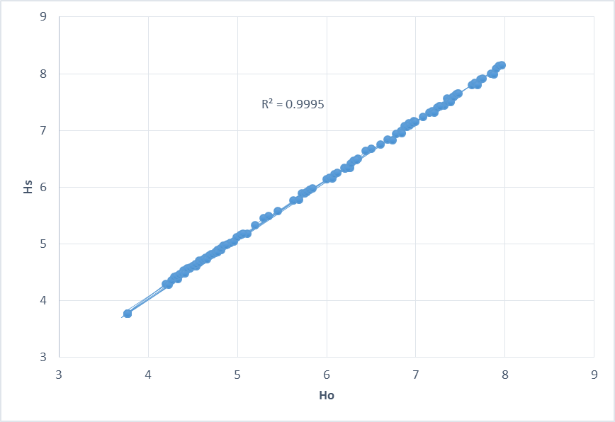
Figure 5: Relationship between observed and simulated hydraulic heads for Observation Wells.
5. Conclusions
In the present study a computer model for a pumping well (discharge well) based on FEM using two slave programs of Geo-Slope software i.e. (SIGMA/W and SEEP/W) has been developed and calibrated. The model has been used to study the behavior of watertable and drawdown in an aquifer during pumping. SIGMA/W program was used to compute initial pore-pressure within an aquifer, while SEEP/W program was used to analysis the change in pore-pressure and drawdown during pumping respectively. To achieve this objective five year old data was depicted in this research. A field experiment was conducted by WAPDA during the year 2011 – 2012 on a homogeneous and anisotropic type unconfined aquifer located over an impervious layer at Tando Soomro, which is 50 km away from Hyderabad, Sindh – Pakistan. The experiment was conducted on a WAPDA installed tube-well (discharge well) along with 5 bore holes at a distance of 900 m, 1,800 m, 3,000 m, 4,800 m, and 5,100 m respectively. The outcome of the research shows that the FEM model consistently yields accurate drawdown in contrast with field observation.
Initially, SIGMA/W program was used to acquire the initial pore-pressure within the aquifer for (t = 0 minutes). The initial pore pressure computed from SIGMA/W was then used by SEEP/W to find out the change in pore-pressure at different depths respectively. The effect of the pumping was analyzed using a steady-state SEEP/W analysis. Boundary conditions was applied on the left and right ends, so that the water level remains at the initial watertable. From the results it is revealed that the vectors displaying the movement of the flow direction towards discharge well due to which decline in watertable occurs and a cone of depression and drawdown curve was formed. Comparison of the experimental data and simulated data showed a good agreement among them. The drawdown line (phreatic line) has been simulated for each concern depth at each interval of time and compared with the actual data and the model demonstrates high efficiency and good fitness.
In order to counter-check the simulation results and to evaluate the performance of numerical model an observed piezometric head difference for all observation wells at different interval of time was finally compared with the simulated piezometric head accordingly. Statistical analysis of all the research data i.e. RMSE, ME, R.E, and EF to evaluate the performance of the model are found to be 0.134 m and 0.126 m, 3.05% and 98.86% respectively. The compared results showed that experimental piezometeric head readings are very close to the simulated readings; however some variation has been observed which may be due to personal errors. Consequently, it is concluded that simulated values of piezometric heads are not much different than the observed readings.
Additionally verifiability of the model is also made by comparing observed and simulated values of piezometeric heads; such graph is illustrated in Figure 5. The slope of the line is observed to be approximately at 45 degree; thus the figure indicates no considerable difference between observed and simulated head values for all the observation wells. Consequently, it is concluded that simulated values of piezometeric heads are not much different than the observed ones. The SIGMA/W and SEEP/W predictions of the pore- pressure distribution during pumping are found to be in very good agreement with the data. The results support the use of these programs as a tool for investigating and designing pumping well practices. Furthermore, as this software is adaptable in nature, therefore it can also be used to solve other types of problems i.e. seepage and slope stability in earthen dams; simulation of phreatic line in earthen dams and other hydraulic structures, modeling of lysimeters, sea water intrusion and other related issues, etc. It should to be introduce in universities and concern institution to gain knowledge about Finite Element modeling and software use.
- Yousafzai, Y. Eckstein, P. Dahl, “Numerical simulation of groundwater flow in the Peshawar intermontane basin, northwest Himalayas”. Hydro. J., 16(7), 1395-1409, 2008. http://dx.doi.org/10.1007/s10040-008-0355-5
- Ashraf, Z. Ahmed, “Regional Groundwater Flow Modeling of Upper Chaj Doab, Indus Basin”, Geophy. J. Int., 173(1), 17-24, 2008. http://dx.doi.org/10.1111/j.1365-246X.2007.03708.x
- Bansal, R. Kumar, J. K. Das, S. Kumar, “Analytical Solution For Transient Hydraulic Head, Flow Rate And Volumetric Exchange In An Aquifer Under Recharge Condition”, J. Hydro. Hydromec., 57(2), 113–120, 2009. http://dx.doi.org/10.2478/v10098-009-0010-4
- Mark, M. Kees, A. J. R. Von, “Calibration of transient groundwater models using time series analysis and moment matching”, Water Reso. Res., 44(1), 1-11, 2008. http://dx.doi.org/10.1029/2007WR006239
- Mehrdad, K. Majid, R. G. Reza, “Inverse modeling of variable-density groundwater flow in a semi-arid area in Iran using a genetic algorithm”, Hydrogeo. J., 2(1) 1-13, 2010. http://dx.doi.org/10.1007/s10040-010-0599-8
- Geo-Slope,” Seepage through A Dam Embankment”. Geo-Slope International Ltd, Calgary, Alberta, Canada, 2007.
- Arshad I., M. M. Baber, “Finite Element Analysis of Seepage through an Earthen Dam by using Geo-Slope (SEEP/W) software”. Int. J. Res., 1(7), 12-16, 2014. Online Access
- Arshad, M. M. Babar, and A. Sarki, “Computation of Seepage Quantity in an Earthen Watercourse by SEEP/W Simulations Case Study: “1R Qaiser Minor” – Tando Jam-Pakistan”. Advan. J. Agric. Res., 3(1), 082-088, 2015. Online Access
- Arshad, “Numerical Analysis of Phosphate Movement through the Sandy Loamy Clayey Soil by CTRAN/W Simulations”. Advan., J. Agric. Res., 3(1) 089-097, 2015. Online Access
- S. Zektser, “Groundwater and the environment: applications for the global community”, Lewis, Boca Raton, Florida, p 175, 2000.
- R. Arora, “Irrigation, Water Power and Water Resources Engineering”. Reprinted Stand. Pub. Distri. Dehli, 6(1) 55-56, 2006.
- M. Alley, and S.A. Leake, “The journey from safe yield to sustainability”, Ground Water, 42(1), 12-16, 2004. http://dx.doi.org/10.1111/j.1745-6584.2004.tb02446.x
- Z. X. Wei, “Temporal and Spatial Discritization on Quasi-3D Groundwater Finite Element Modeling to Avoid Spurious Oscillation”, J. Hydrodyn., 19(1), 68-77, 2007. http://dx.doi.org/10.1016/S1001-6058(07)60030-4