1. Introduction

The maximum flows problem in industrial systems (energy, information or material) can be modeled by graphs’ theory which adequately describe the topology of the studied system [1].

Note: For simplicity of the present analysis, it will be used only the term flow, regardless of type of the studied system – power [2, 3], information [4], communication [5, 6] or transportation [7].

Energy flows are optimized in power systems. In this sense, in [8] a review of the stochastic optimization methods, solving the optimal power flow problem. An application of the graphs’ theory for the energy flows optimization in electric networks is made in [9]. The transformation of the linear model (e. g. linear goal function and linear constraints as unequations) to the directed graph’s model is made there. Thus, the optimization procedure is expressed analyzing the resulting directed graph.

The definition of the flows problem in information systems is made in [10]. In [11] a review of approaches modelling information flow for organizations is presented. A new graph theoretical concept for analyzing the information flows passing through the directed graph’s model, using guessing numbers is proposed in [12].

In [13], the problem of optimization the information flows passing through the uncertain networks with a given constrained capacities of the arcs is considered. The solution bases on the two NP-hard subproblems. First, it calculates the expected information flow associated to a source vertex and next it makes an optimal choice of arcs.

The flows optimization passing through the manifacturing systems is widely discussed issue.  One possible solution to this problem is given by the graph’s theory. For example, in [14] using the shortest path method for flows optimization in cellular manufacturing systems. In [15] an optimization for single-part flow-line configurations of reconfigurable manufacturing systems (RMS) is suggested. In [16] the other optimization approach of the flows in RMS systems is proposed. This approach also uses the graphs’ theory for modeling the considered system. In [17] third model for optimizing demand period cost (fixed plus operating) of RMS flow-line configurations, based also on graphs’ theory, is suggested.

A wide range of problems arise in real-world networks such as Internet, local information networks, energy systems, etc., which are modeled by directed graphs. In [18] a review of a range of theoretical primitives for generating a simple graph based on the given degree sequence is proposed. This is based on the graphs’ theory and the computer networks. Several problems for which efficient algorithms for determining the theoretical solutions are proposed. Since in practice the graphs’ models consists of tens of thousands of vertexes, approximation algorithms are particularly important.

The present paper is organized as follows. In a Section 2 the directed graph’s model with one source – one recipient is defined, as well as the three necessary and sufficient conditions for performing its topological analysis. Five basic tasks arising in real systems, modeled with directed graphs, are also defined. In Section 3 an universal algorithm for solving all these five problems is briefly described. Solutions of these five type of problems applying the universal algorithm is proposed in Section 4. The applicability of this algorithm is visualized in Section 5 on an illustrative example describing problem 1. In the same section, a comparison is made with the obtained solutions to the same illustrative example using traditional methods based on minimum-cut the theorem, such as: Ford Fulkerson, Edmonds Carp and Dinic algorithms. The paper finishes with the conclusion remarks on the universality and advantages of the suggested algorithm.

The novelty of the proposed method consists in its universal application in determining the maximum flow passed through a arbitrary directed graph, whose model contains one initial and one final nodes. It is applicable to analysis of different systems – information, power, manufacturing, etc. The algorithm can be used for solving the five types of problems, defined in the next section

2. Problem statement

The maximum flow problem passing through the arcs of an directed graph is defined in [1].

In order to refine the considered graph’s model, some basic concepts and initial hypotheses will be briefly introduced.

Let’s consider a directed graph , with  vertexes and arcs. The latter is associated to the system’s channels. Let’s   is the  flow passing through the arc . The capacity of this arc is  [4].

A necessary and sufficient condition for determining the maximum flows passing through the arcs of the studied directed graph satisfies the following three assumptions.

Assumption 1

Balance condition: The sum of the incoming flows in a vertex  is equal to the respective sum of the outgoing ones, i.e.

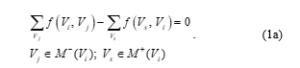
where:      is intermediate vertex for the considered directed graph;

          and are the sets of input and output vertexes for the vertex , respectively.

Assumption 2

Sequencing condition: The flow  passing through the arc  must not exceed its capacity ., i.e.

Assumption 3

Invariability condition: In absolute value, the flow passing through the directed graph from the source vertex to the recepient vertex must be exactly equal to that in the opposite direction.

where   is the  flow passing through the directed graph.

The first condition can be violated if part of the flow is dissipated in a vertex of the graph. This can be observed in the energy transfer, when each vertex is a specific physical device that consumes electricity and at the same time can dissipate it in the form of heat.

The second condition cannot be violated, since real systems are considered where it is physically impossible for a flow to pass through an arc that is greater than its capacity.

In real energy systems there are transfer losses, conversion losses, etc. In this case moving in the both directions of the graph (from the source to the recipient and vice versa) these losses cannot be equal, but they are very close.

Note:  Without a loss of generality it is assumed, that the directed graph’s model of the system has 1 source and 1 recipient vertexes. In general case, it can have multiple sources ( ) and multiple recipients ( ). Then the graph is transformed to a directed graph of the first type by adding fictive source  and recipient vertexes, respectively  (Figure 1).

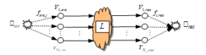
Figure 1: Graph’s model with multiple sources – multiple recipients

In real systems depending on their parameters the following 5 types of maximum flow  problems can be arised. In the first four of them the flow through the arcs  is constant, and in the last one – it varies.

Problem 1: The arcs’ capacities  are known and the capacities of all graph’s vertexes are infinity, i.e. .

Problem 2: The arcs’ capacities  are known and limited in a given range .

Problem 3: The arcs’ capacities     and the capacities  of the graph’s vertexes  are known.

The Problems 1, 2 and 3 discuss the directed graph’s model with one source and one recipient.

Problem 4: It consideres the directed graph with multiple sources  and multiple recipients (Figure 1). The arcs’ capacities    are known.

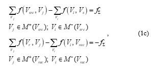
Problem 5: The arc’s capacities  of all the graph’s arcs  are known, but the balance condition (1a) is violated.

where  and  are the input and the output flows, associated to the arc , respectively.

For each of the above defined problem it obtains the maximum  flow passing through the directed graph from the source to the recipient vertexes.

The basic aim and the contribution of the author of this paper consists of the suggesting the universal general algorithm for obtaining the maximum flow started from the source vertex and reached to the final graph’s vertex – either real  or  fictive .

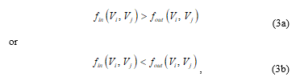
There are always losses when transmitting information or energy through the graph’s model from the source to the recipient.  They decrease the flow , i.e. the condition (3a). The condition (3b) is satisfied in some types of manufacturing systems.

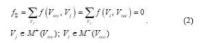
For all 5 maximum flow problems defined above, the condition (1b).

The input flow for the system is generated by the source vertex  and it is named as . The output flow    is the flow, consumed by the recipient . It s assumed that the flow passing through the intermediate graph’s vertexes is zero.

The different types of flows are defined in [1]. For the future analysis, we will describe them again in briefly.

Definition 1:         The allowed flow is:

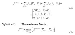
where  are all allowed flows with number i passing through the directed graph from the source to the recipient vertexes.

Definition 3:         The conventionally optimal flow  is, if arbitrary allowed flow satisfies at least one of the conditions (6)

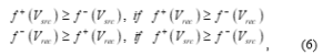
where:  – the flow, generated from the vertex passing through the graph’s model from   to  ;

              – the flow, consumed of the vertex passing through the graph’s model from   to ;

              – the flow, consumed of the vertex passing through the graph’s model from   to  ;

              – the flow, generated from the vertex passing through the graph’s model from   to .

Definition 4:  The maximum allowed flow is , if it satisfies all the conditions (4), (5) and (6) simultaneously.

3. Algorithm of the universal approach for determining the maximum flow problems

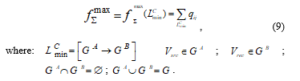
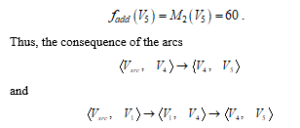
Each problem defined in the previous paragraph can be reduced to the optimization maximum flow problem, where the the goal function is:

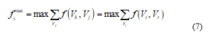
where   is the maximum flow passing through  the minimum intersection  of the considered directed graph.

The basic directed graph, which is divided into two separate ones   and  this function is:

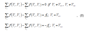
The approach, solving the optimization problem (7) with constraints (8) is proposed and described in details in [19]. Each iteration consists of two procedures – vertexes marking and flows correction. The iteration process stops when the minimal intersection   in the directed graph’s model is determinated.

Before starting the algorithm, it is necessary to know the structure of the directed graph modeling the considered system as well as the capacities of each graph’s arc. It is assumed that the initial values of the flows  passing through the graph’s arcs  are zero.

In Procedure 1 a vertexes marking is made. Each node is assigned the appropriate pair of marks, moving from source to the recipient vertexes. This marking indicates where the respective flow comes from and its maximum allowable value that can be passed through the respective arc. When all vertexes are marked then the algorithm goes to the Procedure 2. This procedure moves from the recipient to the source vertexes correcting the flows passing through each of the arcs in the respective sequences of arcs in the considered directed graph. If all the arcs entering the vertex are saturated, then the maximum flow is determined and the procedure stops. Otherwise it returns to the beginning of Procedure 1.

Note:   An arc is saturated if the flow that passes through it  is exactly equal to its capacity .

4. Solutions to the defined 5 types of the problems

The maximum flow determination approach, proposed in [19], can be applied to solve each of the typical problems, defined in Section 2.

Problem 1

Before starting the algorithm the directed graph’s model is determined. In this model the values of the arcs capacities and vertexes infinity capacities  are known.

To simplify the future exposition and without loss of the generality the maximum flow  is obtained for the intersection of the directed graph’s model shown in Figure 2. For simplicity the elements (vertexes and arcs) included in the beginning of the graph are aggregated in the set .

In this problem the condition (1b) is satisfied, i.e. the flow   passing through the arc , have to be smaller or equal its capacity .

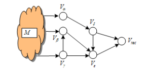
Figure 2: Idealized system described by the graph’s model

Based on the minimum intersection (see Figure 2), which satisfy the condition (4), the respective maximum flows are:

Conclusions:

• The maximum allowed flowis equal to the sum of the capacities of the arcs , because they beyond to the minimum intersection  and they are saturated (their capacity is exhausted).
• The maximum allowed flow for the arc  is equal of the capacity of the arc , because it is assumed that the condition  is satisfied. Therefore, the arc  is saturated and it is added to the minimum intersection .
• The final maximum flow, determined by (4) and Eq. (8) is .

Problem 2

Before starting the algorithm the directed graph’s model is determined. In this model the values of the arcs capacities  are known and each of them must belong to an initially defined range, i.e. .

The solution of the Problem 2 requires a transformation the basic directed graph’s model to the new one, where:

• Each arc is replaced by two new arcs – and .
• The capacity of each of these new arcs determines as follows:
  • about the arc ;
  • about the arc .
  • It introduces the fictive arc with infinity capacity,e. .

Then the Problem 2 has a solution only when the condition  is satisfied.

The transformed graph’s model is the same as in Problem 1. Hence, the maximum flow  is determined in the same way.

Problem 3

Before starting the algorithm, the directed graph’s model is determined. In this model the values of the arcs capacities and vertexes capacities  are known.

The specificity of this problem requires that the additional condition (8) to be included:

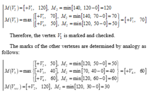
where:     is the flow entering to the vertex ;

 is the set of arcs, which are directly connected with the vertex only by one arc.

To get the solution of this problem it is necessary to transform the basic directed graph’s model to the new one with  vertexes where n and m are the number of vertexes and arcs in the initial directed graph, respectively.

• Each vertex is replaced by two vertexes  and , which are connected by the arc ;
• The capacity of the arc is obtained as follows:

The transformed graph’s model is the same as in Problem 1. Hence, the maximum flow  is determined in the same way.

Problem 4

The initial conditions for this problem are the same as these in Problem 3 with the following additions. Fictive source and receiver are introduced, where each of them is associated with more than one real one (Figure 1). It is assumed that the graph’s vertexes have infinite capacities, i.e. .

The graph’s model from the Problem 4 has vertexes  and  arcs compared to the models in Problems 1, 2 and 3, where n and m are the number of vertexes and arcs in the initial directed graph from Problem 1, respectively.

The resulting graph’s model is the same as in Problem 1. Hence, the maximum flow studied  is determined in the same way.

Problem 5

Before starting the algorithm the directed graph’s model is determined. In this model the values of the arcs capacities and the values of the coefficients , correcting the flow, passed through all of the graph’s arcs are known. The latter are always positive and they reflect to the increasing ( ), resp. decreasing ( ) of the flow in the arc respective .

The next three steps describe the application of the considered heuristic algorithm [19] for solving Problems 1, 2 and 3, resp. 4 and 5, which are reduced to Problem 1.

1. Flows’ ccorrection passing through the graph’s arcs

The flows’ correction is performed in the following way:

Note: If  then the condition (1a) is satisfied and the directed graph’s model is associated to the Problems 1, 2 or 3.

2. Determining the graph’s paths from the source vertex to the recipient vertex , where the resulting flow increases

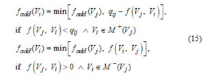
If the conditions

are satisfied, then there is a path from the vertex  to the vertex in the analyzed directed graph, where the resulting flow increases.

The example of this path including two arcs with straight direction and two ones with opposite direction and their capacities  and correcting coefficients , is shown in Figure 3.

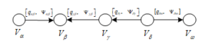
Figure 3: Path with initial vertex  and final vertex , including two straight and two opposite arcs

3. Obtaining the active cycles in directed graph’s model

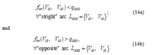
In directed graph’s model  there is an active cycle , connected by the recipient vertex   , if the following conditions are satisfied:

• The value of the summary correcting cycle’s coefficient is bigger than 1, i.e. .
• The cycle’s capacity is not zero, i.e. .
• The cycle includes a vertex , which is directly connected to the recipient vertex .

The example of this type cycle is shown in Figure 4.

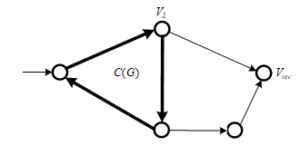
Figure 4: A cycle in directed graph’s model

Note: It is allowed in directed graph’s model to have cycles, connected to the source vertex .

5. Application of the maximum flow suggested approach to an illustrative example about Problem 1

The algorithm for finding the maximum flow [19] will be illustrated for solving the Problem 1. Let’s the following example of the directed graph’s model is analyzed (Figure 5a). On the directed graph the following quantities are indicated:

• The capacities of the respective arc  are shown below it.
• The values of the flows passing through the arc  are underlined and are written above to the arc. It is assumed that the initial values of these flows for all arcs are zeroes.
• The vertexes marks are noted in the following way:
• , with respect to an increasing (+) or decreasing (–) flow passing through the arc ;
• – the maximum value of the additional flow  from the source vertex    to the vertex    passing through the sequence of the arcs, where the flow increases. This flow is determined as follows:

It is assumed that the initial marks of all vertexes are zeroes. And the source vertex  gets the mark , i.e. the generated flow from the source vertex is infinite.

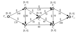
Figure 5a: Illustrative example for solving a maximum flow problem

When applying the heuristic algorithm [19], each iteration consists of 2 steps: first the vertices in the considered directed graph are marked and checked, and second the flows passed through the arcs in the graph’s model are corrected. When marking the vertices, the algorithm moves from the beginning to the end of the graph, and when correcting the flows – vice versa, taking into account the capacity of each arc.

The required maximum flow is determined when all incoming arcs in the end graph’s vertex are saturated. For the present example, this happens to the third iteration. The iterations are following.

Iteration 1

Vertexes marking (Figure 5b)

The source vertex is marked with:

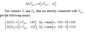
The vertexes  and , that are directly connected with  get the following marks:

Therefore, the vertex  is marked and checked.

Let’s move to the next vertex – , which is marked but not checked. The latter is connected to the vertexes  and . So their marks are determined as follows:

Therefore, the vertex  is marked and checked.

The marks of the other vertexes are determined by analogy as follows:

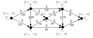
Figure 5b: Results from vertexes marking in an Iteration 1

So, all vertexes in the directed graph are marked and checked.

Flows correction (Figure 5c)

The vertex  is chozen as a start vertex and we move from the end  to the beginning of the directed graph. Using Eq. (11) it determines the flow

                               .

is formed basing on the first mark coefficients of the respective vertexes. Then, using Eq. (12) the corrected values of the flows only in this arcs are calculated as follows:

is satisfied for the arc . Then the arc is saturated and it is marked with bold.

Figure 5c: Results from the flows corrections in the end of an Iteration 1

Since the arcs are not saturated the algorithm passes to next iteration – Iteration 2.

Moving from  to the as a result of this iteration a flow equal to 30 units is passed through each of the arcs .

Iteration 2

Vertexes marking (Figure 5d)

Based on the information from Figure 5c, the new mark of the vertexes is set as follows:

Figure 5d: Results from vertexes marking in an Iteration 2

Flows correction (Figure 5e)

Using Eq. (11) for the arc  the additional flow, is determined:

is formed basing on the first mark coefficients of the respective vertexes. Using Eq. (12) the corrected values of the flows only in these arcs are corrected as follows:

is satisfied.  Then the arc is marked bold.

Based on the additional flow , the corrected flows are:

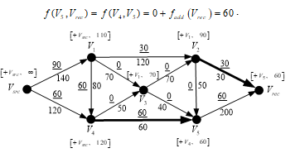
Figure 5e: Results from the flows corrections in the end of the Iteration 2

Since the arcs are not saturated the algorithm passes to next iteration – Iteration 3.

Moving from  to the as a result of this iteration a flow equal to 60 units goes through each of the arcs . This additional flow of 60 units is then added to the current flows through the arcs and , and finally, the flows of 60 and 90 units pass through the arcs, respectively.

Iteration 3

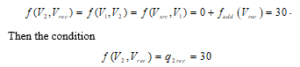
Vertexes marking (Figure 5f)

Based on the information from Figure 5e, the new mark of the vertex  is set as follows (Figure 5f):

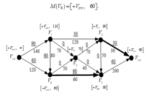
Figure 5f: Results from vertexes marking in an Iteration 3

3.2.         Flows’ correction (Figure 5g)

Using Eq. (11) the arcs and  the following additional flows, are determined:

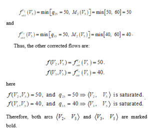
Therefore, both arcs  and  are marked bold.

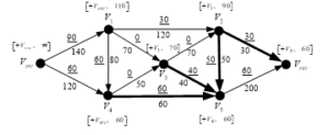
Figure 5g: Results from the flows corrections in the Iteration 3

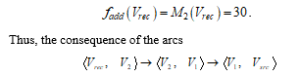
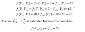
The solution of the maximum flow problem is shown in Figure 5h, where the final vertexes are marked and flows corrections are made:

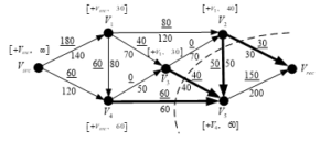
Figure 5h: Final maximum flow

Moving from  to the , as a result of this iteration, the following will happen. First, a flow equal to 40 units is passed through each of the arcs . This additional flow of 40 units is then added to the current flows through the arcs , and finally flows of 130, 40 and 40 units will pass through the arcs, respectively. Second, a flow equal to 50 units is passed through each of the arcs . This additional flow of 30 units is then added to the current flows through the arcs , and finally flows of 180, 50 and 50 units will pass through the arcs. Thus, the resulting flow through the arc will be 180 units.

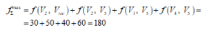
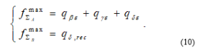
After the last iteration, it is seen that all arcs, where a flow passing through, are saturated. Therefore, an end solution is reached and the final maximum flow is:

In the analyzed illustrative example, the final maximum flow has been found after the third iteration, because all arcs of the cross section shown in Fig. 5h passing flow to the end vertex  are saturated, i.e. the flow passing through them  is exactly equal to the capacity of the corresponding arc .

A comparative study between the discussed heuristic algorithm and a standard min-cut algorithm for solving the maximum flow problem

The obtained solution with a heuristic approach of [19] for an illustrative problem shown in Figure 5a is compared with  analogous ones, determined by traditional methods based on min-cut theorem [20, 21, 22]. The latter is the following: “For any directed weight graph, the maximum flow passed through from the source to the recipient vertex is equal to the capacity of the minimum cut.”. Then it is necessary to obtain the set of arcs with minimum weight that after removing from the graph there is no path from the source to the recipient vertexes. The following methods were used: Ford Fulkerson [23], Edmonds Karp [24] and Dinic algorithms [25, 26]. The calculations are made with free software Visualgo. The final the full solution of the considered problem about the maximum flow is obtained.

Note:  In contrast to the method applied in this article, in the final solution Visualgo visualizes the flow that passes through each of the arcs and their remaining capacity, depending on the full arc’s capacity, as shown in Figures 5a-5h.

The final solution obtained through the used methods are shown in Figures 6a, 6b and 6c.

Figure 6a: Final maximum flow obtained by the Ford-Fulkerson’s algorithm

Figure 6b: Final maximum flow obtained by the Edmonds-Karp’s algorithm

Figure 6c: Final maximum flow problem obtained by the Dinic’s algorithm

The final maximum flow, determined by these three methods, based on min-cut theorem (Figures 6a, 6b and 6c), are the same as those of the heuristic approach applied in this article:

The advantage of the proposed approach is that the final solution is obtained on the 3^rd iteration, and each iteration consists of two procedures.

In the method of Ford Fulkerson, the final solution is obtained on the 6^th iteration. The Edmonds Karp algorithm consists of two built-in cycles. For the considered example the final solution is obtained on the 4^th iteration. As the external cycle is executed 4 times and each time from its execution the internal is executed only once. The Dinic algorithm consists of two build-in cycles. For the considered example the final solution is determined after applying the external cycle 2 times. Initially, the internal cycle is rotated 2 times after that – it rotates 3 times. All this shows the better efficiency of the proposed algorithm

6. Conclusion

Determining the maximum flow and the distribution of the flows in the analyzed directed graph based on the interconnections in its topology is an important prerequisite for the efficient use of resources in the considered system. The solution of this optimization problem depends on the structure of the comsidered graph’s model and the capacities of its arcs. The heuristic approach used in this article is universal not only in terms of the physical nature of the studied system, but also in terms of different types of problems considered –  the input data of each of analyzed problem are different.

The solutions to the Problems 1, 2, 3 and 4 show that the flows passing through the arcs of the graph’s model are constant. The solution to the Problem 5, however, shows that the flow is variable, so one can make a general conclusion when the new approach has been successfully applied in the case of violation of the balance condition.

In the present paper, the results of the solution for Problem 1 with heuristic algorithm are compared with these obtained from other analogous methods:  Ford-Fulkerson’s, Edmonds-Karp’s and Dinic’s algorithms. The time complexity of this algorithm is equal to that of the Ford-Fulkerson’s and Edmonds-Karp’s algorithms – , in contrast to that of the Dinic’s algorithm, where it is . The illustrative example shows that it is faster to converge to the final solution comparing to the other considered algorithms.

The used universal algorithm is inapplicable to solving problems in which at least one of the three initial assumptions (defined in Problem statement) is not fulfilled, i.e. Balance condition, second condition for sequencing the flow passing through the arbitrary arc with its capacity and third condition for the invariability of the flow passing through the considered graph moving from the source to the recipient vertexes and vice versa.

One of the possible future development of the work is related to the program realization of the proposed approach for determining the maximum flow passing through a directed graph.

Other trend for the future development of the research on solving this problem is using an algorithm based on determining all possible paths in the considered directed graph, proposed in [27]. It uses two adjacent matrices corresponding to each vertex of the graph – these of the input and output arcs in the vertex, respectively. As a result of the algorithm, one will only be interested in the maximum flow that has passed the shortest path from the start to the end vertex in the directed graph.

Conflict of Interest

The author declares no conflict of interest.

Acknowledgment

The publication of this manuscript was realized by financial support from the Scientific Research Sector of the Technical University of Sofia.

1. H. A. Taha, Operations research: An introduction, Prentice Hall Price, 2017.
2. J. A. Bondy, Murty, U. S. R., Graph Theory, Springer, 2008.
3. N. Sayeekumar, Sh. Ahmed, S. Karthikeyan, S. Sahoo, I. Jacob, “Graph theory and its applications in power systems – a review”, in 2015 IEEE International Conference on Control, Instrumentation, Communication and Computational Technologies (ICCICCT), 18-19 Dec. 2015, doi: 10.1109/ICCICCT.2015.7475267.
4. J. Burch, Grudnitski, Information system. Theory and Practice, John Wiley & Sohn, 1997.
5. S. L. Hakimi, “Application of graphs theory to problems in communication systems and networks”, AD-A030 888. U. S. department of Commerce, National Technical Information Service, Northwestern Univ. Evenston III, Dept. of Electrical engineering, Air Force Office of Scientific Research, Boiling AFB, D C. 1976.
6. G. Cherneva, H. Spiridonova, “Matching Filters Design for Information Transmit in Power Line Communication Systems”, Mechanics, Transport, Communications Journal, 3/2, ХI-21- ХI-27,3/2,  2018, (in Bulgarian).
7. S. Guze, “Graph Theory Approach to Transportation Systems Design and Optimization”, International Journal on Marine Navigation and Safety of Sea Transportation, 8(3), Dec. 2014, doi: 10.12716/1001.08.04.12
8. V. Radziukynas, I. Radziukyniene, Optimization Methods Application to Optimal Power Flow in Electric Power Systems, Optimization in the Energy Industry, Chapter 18, 409-436, Jan. 2009, doi: 10.1007/978-3-540-88965-6_18
9. P. H. Nguyen, W. L. Kling, G. Georgiadis, M. Papatriantafilou, L. A. Tuan, L. Bertling, Application of the Graph Theory in Managing Power Flows in Future Electric Networks, New Frontiers in Graph Theory, Chapter 12, March 2012, doi: 10.5772/35527
10. Schade, M. Begley. “Information flow diagram guidelines”, 23 Sept. 2012, retrieved 20 March 2016.
11. D. Christopher, T. Ashutosh, A. R. Jeffrey, “Modelling information flow for organisations: a review of approaches and future challenges”, International Journal of Information Management, 33(3), 597–610, June 2013, doi:10.1016/j.ijinfomgt.2013.01.009
12. S. Riis, “Information flows, graphs and their guessing numbers”, in 2006 IEEE 4th International Symposium on Modeling and Optimization in Mobile, Ad Hoc and Wireless Networks, 26 Feb. – 2 March 2006, doi: 10.1109/WIOPT.2006.1666516.
13. Ch. Frey, A. Zufle, T. Emrich, M. Renz, “Efficient Information Flow Maximization in Probabilistic Graphs”, IEEE Transactions on Knowledge & Data Engineering, 30(5), 880-894, 2018, doi:10.1109/TKDE.2017.2780123
14. K. A. Prasath, R. D. J. Johnson, “Fundamental Approach on Layout Optimization Using Graph Theory in Cellular Manufacturing Systems”, Australian Journal of Basic and Applied Sciences, 9(33):180, October 2015.
15. J. Dou, X.-Z. Dai, Z.-D. Meng, J. Li, “Optimization for single-part flow-line configurations of reconfigurable manufacturing system based on graph theory”, Jisuanji Jicheng Zhizao Xitong/Computer Integrated Manufacturing Systems, CIMS, 16(1), 81-89, 2010.
16. J. Dou, X. Dai, Zh. Meng “Graph theory-based approach to optimize single-product flow-line configurations of RMS”, International Journal of Advanced Manufacturing Technologies, 41, 916–931, 2009, doi: 10.1007/s00170-008-1541-2
17. J. Dou, X. Dai, Zh. Meng, “Optimization for Flow-Line Configurations of RMS Based on Graph Theory”, in 2007 International Conference on Mechatronics and Automation, 1261-1266, doi: 10.1109/ICMA.2007.4303730
18. M. Mihail, N. Vishnoi, “On Generating Graphs with Prescribed Vertex Degrees for Complex Network Modeling”, College of Computing Georgia Institute of Technology, 2002.
19. S. Filipova-Petrakieva, “A New Universal Optimization Approach for Maximum Flows in Power Systems”, in 2019 IEEE XI International Conference BulEF’2019, 11-14.09.2019, doi: 10.1109/BulEF48056.2019.9030731
20. G. B. Dantzig, D. R. Fulkerson, “On the Max-Flow MinCut Theorem of Networks”, in Linear Inequalities, Ann. Math. Studies, no. 38, Princeton, New Jersey, 1956.
21. G. B. Dantzig, D.R. Fulkerson, “On the max-flow min-cut theorem of networks”, RAND corporation: 13, 9 September 1964, retrieved 10 January 2018.
22. G. Eusden, “Max-Flow, Min-Cut – History and Concepts Behind the Max-Flow, Min-Cut Theorem in Graph Theory”, 2013.
23. L. R. Ford, D. R. Fulkerson, “Maximal flow through a network”, Canadian Journal of Mathematics, 8, 399–404, 1956, doi: 10.4153/CJM-1956-045-5.
24. J. Edmonds, R. M. Karp, “Theoretical improvements in algorithmic efficiency for network flow problems”, Journal of the ACM, 19(2), 248–264, 1972, doi:10.1145/321694.321699.
25. E. A. Dinic, “Algorithm for solution of a problem of maximum flow in a network with power estimation”, Soviet Mathematics – Doklady, Doklady, 11, 1277–1280, 1970.
26. Y. Dinitz, “Dinitz’ Algorithm: The Original Version and Even’s Version”, In Oded Goldreich; Arnold L. Rosenberg; Alan L. Selman (eds.). Theoretical Computer Science: Essays in Memory of Shimon Even, Springer, 218–240, 2006.
27. V. M. Mladenov, Kr. N. Filipova, S. K. Petrakieva, B. Dimov, H. Uhlmann, “Analysis of Signal Competition in Asynchronous Ultra High-Speed Digital Circuits”, Przeglad Elektrotechniczny (Electrical Review), 83(11), 197-200, 2007.

(Click Here)

(Click Here)