1. Introduction

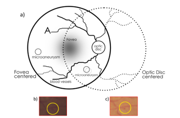
This paper is an extension of the algorithm originally presented in the International Conference on Signal Processing Theory and Applications (IPTA 2016) [1]. This work adds a combination of spatial information from two retinal images for microaneurysm (MA) detection. Diabetic Retinopathy (DR) is one of the most common causes of blindness among working-age adults [2]. Signs of DR can be detected from images of the retina which are captured using a fundus camera. Microaneurysms (MAs) are one of the early signs of DR. Several algorithms for automated MA detection from single 45 degree fundus images have been proposed in the literature. However, in many Diabetic Eye Screening Programmes, including the UK National Health Service Diabetic Eye Screening Programme (NHS DESP) [3], at least 2 views of the retina are captured including both optic disc centered view and the fovea centered images (Figure 1). These images overlap together and thus have common MAs that appear in both views (with variability in contrast). Despite the availability of both views, the algorithms that have been proposed have only taken into account the information contained in a single image. In this paper an increase in detection accuracy is achieved by fusing the information from two views of the retina.

Algorithms reported in the literature lie broadly in two categories: supervised and unsupervised techniques. Supervised techniques make use of a classifier to reduce the number of false detections. This classifier requires training on an additional training set in order to generate a classification model. Unsupervised methods do not require a classifier and hence no training step is needed.

The majority of the proposed methods in the literature fall under the supervised category. Most of the algorithms consist of three main stages: 1) Preprocessing 2) MA Candidate Detection and 3) Classification. The preprocessing phase corrects the image with respect to non-uniform illumination and enhances MA contrast. MA Candidate Detection detects an initial set of candidates that are suspected to be MAs. While it is possible to stop here and report the detected results, a third phase is usually included in the algorithm to reduce the amount of false positives. This is the candidate classification phase and it classifies the detected candidates from phase 2 as either true or spurious.

A variety of classification techniques have been reported in the literature such as Linear Discriminant Analysis (LDA) [4] K-Nearest Neighbours (KNN) [5]–[8], Artificial Neural Networks [9], [10], Naive Bayes [11] and Logistic Regression [12]. There are a number of unsupervised methods that do not rely on a classifier include [13]–[16]. The obvious advantage of an unsupervised method is that they do not require a training phase. Some initial candidate detection methods that have been proposed are Gaussian filters [4]–[6] or their variants [8], [17], [18], simple thresholding  [15], [16], [19], Moat operator [20], double ring filter [9], mixture model-based clustering [21] 1D scan lines [13], [14], extended minima transform [11], [22], Hessian matrix Eigenvalues [7], [23], Frangi-based filters [24] and hit-or-miss transform [10].

All the aforementioned methods were based on detection from a single colour image. Even though extra information may be available from another view of the retina, these algorithms are not designed to incorporate this extra information. A few methods have addressed the problem of detecting or measuring change from multiple images for the purpose of disease identification. Conor [25] performed vessel segmentation on a series of fundus images and measured both vessel tortuosity and width in these images. This was done in order to find a correlation between these measures and some signs including Diabetic Retinopathy. Arpenik [26] used fractal analysis to distinguish between normal and  abnormal vascular structures in a human retina. Patterson [27] developed a statistical approach for quantifying change in the optic nerve head topography using a Heidelberg Retinal Tomograph (HRT). This was done for measuring disease progression in glaucoma patients. Artes [28] reported on the temporal relationship between visual field and optic disc changes in glaucoma patients. Bursell [29] investigated the difference in blood flow changes between insulin-dependent diabetes mellitus (IDDM) patients compared to healthy patients in video fluorescein angiography. Narasimha [30] used longitudinal change analysis to detect non-vascular anomalies such as exudates and microaneurysms. A Bayesian classifier is used to detect changes in image colour. A “redness” increase indicates the appearance of microaneurysms. Similarly, an increase in white or yellow indicates the appearance of exudates. While the problem of analysing “change” and “progression” of disease has been studied in the literature, to the best of our knowledge, the combination of a spatial pair of retinal images for the improvement of detection of MAs has not yet been explored.

The objectives of the present work are: 1) To present a novel method for combining information from two views of the retina (optic disc centered and fovea centered) and 2) Evaluate this method using a dataset of spatial image pairs. Following this introductory section, the methodology of the proposed method will be explained. Section 3 will discuss the details of the dataset and the methods employed for evaluating the proposed method. Results will be presented and discussed in Section 4. Final remarks and conclusions will be presented in Section 5.

2. Methodology

2.1.  Method Overview

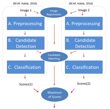
Figure 2 illustrates the overview of the proposed method. A way to compare MA candidate detection using the combined image versus the 2 singular images from the same patient was needed. A previous method [1] was used for the detection of candidates and measuring the probability of each candidate being true or spurious. The method was explained in detail in [1] and will be summarised in the following paragraph.

The previous method worked on the detection of microaneurysms from a single colour fundus image. The method was based on 3 stages: Preprocessing, MA candidate detection and classification. In the preprocessing phases, noise removal was performed and the image was corrected for non-uniform illumination by subtracting it from an estimate of the background. Salt and pepper noise was also removed during this stage. The vessel structure was removed from the image since vessel cross sections usually cause many false positive candidate detections. In the MA candidate detection phase a Gaussian filter response was thresholded in order to receive a set of potential candidates. Each candidate was region grown in order to enhance the shape of the candidates (to match the original shape in the image). Finally, during the classification stage, each region grown candidate was assigned a probability  between 0 and 1 representing the classifier’s confidence in it being a true candidate or not. Each probability  can be thresholded at an operating point  to produce  such that:

Where  means that the corresponding candidate will be classified as true and  means it will be classified as spurious and removed from the candidates set.

The previous method has been adapted to work on 2 images of different spatial views. As shown in Figure 2, the 2 images are run through the algorithm as normal. This produces a set of 2 scores (scores⁽¹⁾ and scores⁽²⁾). The intention is to combine these 2 scores together. However, before fusing the scores a way to find correspondences between candidates is needed. Therefore the images need to be aligned first (Image Registration) and then finding a match between corresponding candidates is needed (Candidates Matching). Each of the matched candidate’s scores can then be combined to produce a single set of scores for both images. This combination should increase the confidence in some true MA candidates, and will hence improve the final algorithm after the final scores are thresholded with an operating point .

In the following sections the Image Registration, Candidates, Matching and Fusion of Scores stages are described in greater detail.

2.2.  Image Registration

Image registration is the process of aligning two images so that their corresponding pixels lie in the same space. One image is considered to be the reference image and the other image (known as the moving image) is transformed to be aligned to the reference image. A global transformation model was used which means that a single transformation was applied across the entire moving image. This has the advantage of simplicity and efficiency, but may not be as accurate as localised registration techniques. Since the goal of this paper was to introduce a proof of concept with regards to combining spatial information during microaneurysm detection, the accuracy achieved was sufficient for this purpose. More accurate registration techniques will be investigated in future work.

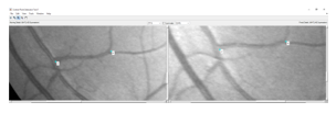
A manual registration technique was employed where corresponding ‘control points’ were selected from each image. These control points were used to solve the global transformation model equations and find the transformation parameters (Figure 3). Corresponding points were annotated in each pair of images (as specified by Table 1).

Based on the literature, four transformation models were evaluated: These include Similarity [31], Affine [32], [33], Polynomial [34], [35] and RADIC [36], [37].

The transformation model parameters were estimated using the six control points that were manually selected on each pair of images. These control points were picked on each image’s vessel cross sections since it was easiest to identify corresponding points at these areas. Figure 4 shows samples of checkerboard patches selected at random from the registered image pairs. In general it was difficult to identify the most accurately registered model by visual observation of the patches alone since there was an observed discrepancy in performance across rows.

In other words, none of the transformation models perfectly aligns the vessels in all four patches. Hence, a more objective method for selecting the model was needed. This will be discussed in Section 3.2.1.

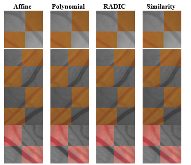
Table 1 The number of control points needed for each transformation model

Transformation model	No. of control points needed
Similarity	2
Affine	3
Polynomial	6
RADIC	3

2.3.  Candidates Matching

Once both images were aligned the candidates detected from both images lie in the same coordinate space and hence can be matched by their location. In order to account for some inaccuracies in the registration, we used the following method to find matches between 2 candidates:

Given two aligned images  and , each candidate  detected in  needs to be matched to one of the candidates detected in . We start by finding the centre of candidate  and define a circular search region with radius  around . A match is made with the candidate in  whose center lies closest to . If no candidate in  is found in this region, no match will be made. This procedure is repeated for all candidates in . In our case we defined  to be 15 pixels which is twice the size of an average candidate in our dataset (Figure 5). This offers more tolerance to account for potential inaccuracies in the image registration.

More formally, let  be the set of candidates detected from the image  and  be the set of candidates detected from image . Our goal is to find a set of correspondences  (where  and ) which represent the correspondences between these candidates. Note that some candidates would not have any correspondences and in this case they would not be a member of any set pair in . In practice either  or  are picked as a ‘reference set’ and matches are found from the other set. For instance, if we pick  as a reference then for each  we find a corresponding match from  and add it to  if any exists. But we would not do vice versa –  would not be used as a reference, and this is done for consistency, since we want to have consistent matches in order to make the fused scores

r

consistent.

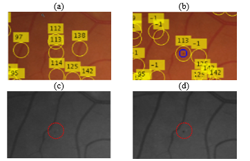
Figure 6 shows an example of correspondences found after following the procedure above. The first row in the figure (a, b) shows a colour image pair while the second row in the figure (c,d) represents the green channel extracted from each image in the first row. Note that the candidates are matched from the image on the right column (b, d) to the image on the left column (a, c). The annotation numbers represent the matches from  to  (A visual representation of ). Candidates annotated with “-1” in the right image represent a candidate that has no correspondence in the other image (no match found in ). The blue circle in the figure represents a true candidate. It can be seen that a match has been found between the true candidate in (b) and its corresponding candidate in (a). Furthermore, it is observed that the candidate has a much higher contrast in the right image than it does on the left one. The MA candidate is still visible in the left image but it much more subtle. Nevertheless, a combination of information from both candidates will give us higher confidence that is a true candidate.

In fact, human retinal graders often switch between both views of the retina when they have suspicions regarding one candidate. The existence of signs in both images would give graders more confidence about it being a microaneurysm. The process of matching in the proposed method attempts to replicate this.

2.4.  Scores Fusion

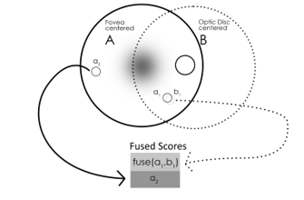
Given that correspondences have been established between candidates and that each classifier has produced scores for each candidate we now need to find a final fused set of scores that represent a combination of information from both images. Suppose we have two matched candidates  and  from images  and  respectively. Furthermore, assume that  is our reference image –i.e. we are currently interested to classify the candidates in . We define the function  as follows (Figure 7):

Where  and  are algorithm parameters specified between 0 and 1. In other words, given 2 matching candidates, the maximum of both their scores is taken only if  lies between the two threshold parameters (  and ). The parameters   and  are used to limit the number of false candidates that get their scores maximized in the final set. This is because maximization of scores should only be done for true candidates

If a candidate in a reference image has no match in the other image then its score is simply copied over to the fused set (Figure 7). Once the fused score set is computed we can perform a final threshold at an operating point  to find the final set of classifications as described in Section 2.1.

3. Results

3.1.  Dataset

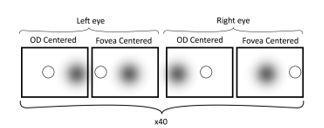
The dataset used for evaluation consists of 40 patients imaged imaged as a part of UK NHS DESP. 4 images are available for each patient: fovea and optic disc centered images for 2 eyes. Hence there are 4 images per patient. The total amount of images is 160 images (Figure 8). The images were captured using different fundus cameras (including Canon 2CR, EOS and Topcon cameras) and hence were of different resolutions (Table 2) however they all had the same aspect ratio of 1.5. Moreover all the images had the same field of view (45 degrees).

The images in the dataset were split into 80 images for training the model and 80 images for validating it. The training set consisted of 112 MAs and the testing set consisted of 95 MAs.

Research Governance approval was obtained.  Images were pseudonymized, and no change in the clinical pathway occurred.

The same test set was used to validate both the proposed technique that takes into account spatial information and the normal technique. The classifier model was generated using the training set and the same model was used for both cases of with and without spatial information. To clarify, the same model was used to generate the scores for both the single-image method and the spatial-information method.

Table 2 The image resolutions of the dataset. All the images had an aspect ratio of 1.5.

Image Resolution	Count
3888 x 2592	24
2592 x 1728	48
3872 x 2592	12
4752 x 3168	32
4288 x 2848	20
3504 x 2336	24
TOTAL	160

 

3.2.  Evaluation

In this section details regarding the evaluation of the registration transformation model and spatial information combination phases are presented. Section 3.2.1 details the selection of the appropriate transformation model objectively. Section 3.2.2 will describe the process for evaluating the spatial information combination and present its results.

3.2.1.         Registration

As shown in Figure 4 it is difficult to decide which transformation model achieves best performance. Therefore we need a more objective measure of registration performance. During the registration we have a reference image  and a moving image  which is transformed to be in the coordinate space of . After the image is transformed to the coordinate space of  we define an overlapping region as all the pixel coordinates where both  and  exist (overlap).

The Centreline Error Measure (CEM) [36] quantifies the mean of the minimum distance between each pixel along the centreline of the reference image and the closest pixel in the moving image. Given a set of coordinates in the reference image that lie on its vessel centreline (Figure 9) and are on the overlapping region of the two images: V= . Similarly, let U=  be the set of points on the moving image that lie on its vessel centreline and belong to the overlapping region. Let  be a transformation that transforms a point  from the moving image space to the reference space. We calculate the centreline error metric for a transformation    on the moving image as follows:

Where  represents the Euclidean distance between coordinates  and . Therefore the CEM calculates the average distance between each point on the reference image and the nearest points on the registered moving image (in the overlapping region).

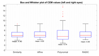
A box and whisker plot of CEM values for each registration model in the same view was plotted in Figure 10. This plot is helpful to summarize the data since it shows the median value and the spread of the values (upper-quartile, lower quartile and the highest and lowest value). Based on this plot it is observed that while the polynomial model contains some of the lowest CEM values (highest accuracy) compared to other models, the distribution of its values also contain the highest spread (as can be seen by the height of the polynomial ‘box’, as well as the highest and lowest values). This can also be seen by the number of outliers in the polynomial plot. This high variance in values is also expressed by the standard deviation of the values as can be seen in Table 3. This suggests the undesirable “instability” of the polynomial model. We also see that the lowest standard deviation values are exhibited by both the affine and the similarity models (with the similarity model having a slightly lower standard deviation). Both the mean and standard deviations of these models are similar to each other which makes their performance comparable. The similarity model was selected since its values exhibited the lowest standard deviation.

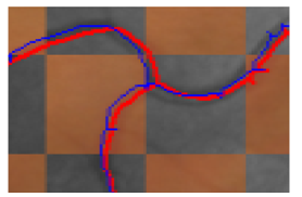
Table 3 Centerline Error Metric (CEM) mean and standard deviation values for various transformation models. Std – Standard deviation.

	Similarity	Affine	Polynomial	RADIC
Mean	4.40	4.50	4.74	4.49
Std	1.51	1.536	3.82	1.536

3.2.2.         Spatial information combination

The method for fusing the scores has been discussed in Section 2.4. In order to evaluate the effectiveness of this method we need a baseline method to compare against. The baselines in our case would be the original proposed method that detects the candidates from a single image [1]. The goal was to provide a direct comparison between the performance when spatial information is accounted for and when it is not accounted for. The method used to compare [1] with the proposed method of this paper was as follows:

• A tree ensemble model was generated using the training set.
• Features were generated from the validation set and the ensemble model (decision tree ensemble) was used to assign scores to each candidate in the 80 images of the validation set.
• In the case of the original image that used single images, an FROC (Free-Receiver operating) curve [38] was generated using these scores alone. This is the solid curve in Figure 11.
• To incorporate spatial information, each image pair (optic disc centered and fovea centered) had their corresponding candidate scores fused as explained in the methodology section. The fused scores were then evaluated collectively for each image pair and this was used to generate the FROC curve in Figure 11.

The parameters for scores fusion were  and . Automating the process of selecting these parameters is left for future work. We see a slight increase after spatial information is incorporated. This increase can be captured quantitatively using the ROC score measure [39]. This score measures the sensitivity values at various x-axis intervals. The measured ROC score shows an increase of 0.02 after adding spatial information, which is a 2% increase. This increase can be explained intuitively as follows: Some candidates appear very subtle in the optic disc centered image, especially at the edge towards around the fovea region. This is because the retina is spherical and would get distorted during image acquisition. This distortion would affect the candidates towards the edge of the image. But these same candidates would appear more clearly in the Fovea centered image. This is because the same candidates now lie in the centre of the captured image, and hence their appearance will be obvious in the image. Intuitively, we expect the classifier to give higher scores to the more obvious candidates in terms of appearance. However, when the scores are fused, we take the maximum score of both candidates, and this will give us a higher score for the more subtle candidate that was originally given a lower score. This is why the FROC curve for the fused candidates shows a better performance.

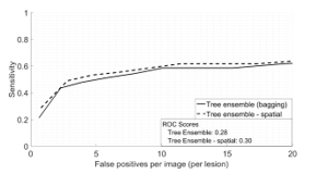
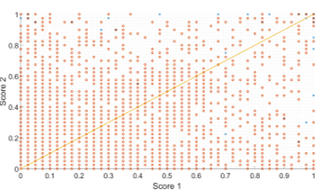
Figure 12 shows this intuitive concept by showing a plot of the corresponding pairs of scores. The figure shows a correspondence of scores for the test set where “score 1” and “score 2” on the axes refer to the methodology scores in Figure 2. Furthermore true candidates are labelled in blue while false detections are labelled in orange. Let us assume Score 2 is the reference image and that the candidate scores are being matched to score 1. Since in our case  and  we are only interested in this cross section from the score 2 axis. If we look to the extreme right of the graph we will see some candidates that have received scores within this range in the score 2. These receive higher scores along the x-axis. Hence, the maximum of both scores in the fused set will improve their scores and this will result in a higher FROC curve.

The additional processing involved is the time for Image Registration, Candidates Matching and Score Fusion. These are the blue ellipse stages in Figure 2. The image registration is dependent on the algorithm of choice. In this work since it is based on manual control points the overhead is the control point selection and the time to solve a series of equations. An automated registration method may require an optimisation step and hence more time will be required for this step [40]. Given a spatial image pair, let  be the number of candidates detected in one image, and  be the number of candidates detected in the other image. The candidates matching step requires calculating the distance between each pairs of candidates detected in both images and hence has a complexity of  (using Big O notation). The Score Fusion phase will fuse the scores together from one image (  fusions) and then fuse the scores from the other image (  fusions) and therefore will have a complexity of . In practice, on a core i5-4590 @ 3.30GHz CPU with 8GB RAM and an SSD hard drive, the time per image for each of the three stages was as follows:

1. Image Registration: 0.02 s
2. Candidates Matching: 1.30s
3. Scores fusion: 0.001s.

The sum of the above timings is 1.321s. The total time for test dataset was computed and then the average value per image pair was found. The average time per pair for the entire process was 4.141s. This means that the average overhead is about 32% of the time required per image (1.321s out of 4.141s). This does not take into account the time for manual control point selection, however, automated registration will be implemented in future work. Methods for optimising the speeds of the other stages are also left for future work.

 

Conflict of Interest

The authors declare no conflict of interest.

Acknowledgment

This work is funded by an internal Scholarship, awarded by the Faculty of Science, Engineering and Computing, Kingston University.

1. M. Habib, R. A. Welikala, A. Hoppe, C. G. Owen, A. R. Rudnicka, and S. A. Barman, “Microaneurysm Detection in Retinal Images Using an Ensemble Classifier,” presented at the The Sixth International Conference on Image Processing Theory, Tools and Applications, Oulu, Finland, 2016.
2. G. Liew, M. Michaelides, and C. Bunce, “A comparison of the causes of blindness certifications in England and Wales in working age adults (16–64 years), 1999–2000 with 2009–2010,” BMJ Open, vol. 4, no. 2, p. e004015, Feb. 2014.
3. “Diabetic Eye Screening Feature Based Grading Forms.” [Online]. Available: https://www.gov.uk/government/uploads/system/uploads/attachment_data/file/402295/Feature_Based_Grading_Forms_V1_4_1Nov12_SSG.pdf. [Accessed: 02-Apr-2017].
4. L. Streeter and M. J. Cree, “Microaneurysm detection in colour fundus images,” Image Vis. Comput N. Z., pp. 280–284, 2003.
5. M. Niemeijer, B. van Ginneken, J. Staal, M. S. A. Suttorp-Schulten, and M. D. Abramoff, “Automatic detection of red lesions in digital color fundus photographs,” IEEE Trans. Med. Imaging, vol. 24, no. 5, pp. 584–592, May 2005.
6. A. D. Fleming, S. Philip, K. A. Goatman, J. A. Olson, and P. F. Sharp, “Automated microaneurysm detection using local contrast normalization and local vessel detection,” IEEE Trans. Med. Imaging, vol. 25, no. 9, pp. 1223–1232, Sep. 2006.
7. K. M. Adal, D. Sidibé, S. Ali, E. Chaum, T. P. Karnowski, and F. Mériaudeau, “Automated detection of microaneurysms using scale-adapted blob analysis and semi-supervised learning,” Comput. Methods Programs Biomed., vol. 114, no. 1, pp. 1–10, Apr. 2014.
8. J. Wu, J. Xin, L. Hong, J. You, and N. Zheng, “New hierarchical approach for microaneurysms detection with matched filter and machine learning,” in Engineering in Medicine and Biology Society (EMBC), 2015 37th Annual International Conference of the IEEE, 2015, pp. 4322–4325.
9. A. Mizutani, C. Muramatsu, Y. Hatanaka, S. Suemori, T. Hara, and H. Fujita, “Automated microaneurysm detection method based on double ring filter in retinal fundus images,” 2009, p. 72601N.
10. R. Rosas-Romero, J. Martínez-Carballido, J. Hernández-Capistrán, and L. J. Uribe-Valencia, “A method to assist in the diagnosis of early diabetic retinopathy: Image processing applied to detection of microaneurysms in fundus images,” Comput. Med. Imaging Graph., vol. 44, pp. 41–53, Sep. 2015.
11. A. Sopharak, B. Uyyanonvara, and S. Barman, “Simple hybrid method for fine microaneurysm detection from non-dilated diabetic retinopathy retinal images,” Comput. Med. Imaging Graph., vol. 37, no. 5, pp. 394–402, 2013.
12. M. García, M. I. López, D. Álvarez, and R. Hornero, “Assessment of four neural network based classifiers to automatically detect red lesions in retinal images,” Med. Eng. Phys., vol. 32, no. 10, pp. 1085–1093, Dec. 2010.
13. I. Lazar and A. Hajdu, “Microaneurysm detection in retinal images using a rotating cross-section based model,” in 2011 IEEE International Symposium on Biomedical Imaging: From Nano to Macro, 2011, pp. 1405–1409.
14. I. Lazar and A. Hajdu, “Retinal Microaneurysm Detection Through Local Rotating Cross-Section Profile Analysis,” IEEE Trans. Med. Imaging, vol. 32, no. 2, pp. 400–407, Feb. 2013.
15. L. Giancardo, F. Mériaudeau, T. P. Karnowski, K. W. Tobin, Y. Li, and E. Chaum, “Microaneurysms detection with the radon cliff operator in retinal fundus images,” in SPIE Medical Imaging, 2010, p. 76230U–76230U.
16. L. Giancardo, F. Meriaudeau, T. P. Karnowski, Y. Li, K. W. Tobin Jr, and E. Chaum, “Microaneurysm detection with radon transform-based classification on retina images,” in Engineering in Medicine and Biology Society, EMBC, 2011 Annual International Conference of the IEEE, 2011, pp. 5939–5942.
17. B. Zhang, X. Wu, J. You, Q. Li, and F. Karray, “Detection of microaneurysms using multi-scale correlation coefficients,” Pattern Recognit., vol. 43, no. 6, pp. 2237–2248, Jun. 2010.
18. Q. Li, R. Lu, S. Miao, and J. You, “Detection of microaneurysms in color retinal images using multi-orientation sum of matched filter,” in Proc. of the 3rd International Conference on Multimedia Technology, 2013.
19. J. H. Hipwell, F. Strachan, J. A. Olson, K. C. McHardy, P. F. Sharp, and J. V. Forrester, “Automated detection of microaneurysms in digital red-free photographs: a diabetic retinopathy screening tool,” Diabet. Med., vol. 17, no. 8, pp. 588–594, Aug. 2000.
20. C. Sinthanayothin et al., “Automated detection of diabetic retinopathy on digital fundus images,” Diabet. Med., vol. 19, no. 2, pp. 105–112, Feb. 2002.
21. C. I. Sánchez, R. Hornero, A. Mayo, and M. García, “Mixture model-based clustering and logistic regression for automatic detection of microaneurysms in retinal images,” in SPIE medical imaging, 2009, vol. 7260, p. 72601M–72601M–8.
22. A. Sopharak, B. Uyyanonvara, and S. Barman, “Automatic microaneurysm detection from non-dilated diabetic retinopathy retinal images using mathematical morphology methods,” IAENG Int. J. Comput. Sci., vol. 38, no. 3, pp. 295–301, 2011.
23. T. Inoue, Y. Hatanaka, S. Okumura, C. Muramatsu, and H. Fujita, “Automated microaneurysm detection method based on eigenvalue analysis using hessian matrix in retinal fundus images,” in Engineering in Medicine and Biology Society (EMBC), 2013 35th Annual International Conference of the IEEE, 2013, pp. 5873–5876.
24. R. Srivastava, D. W. Wong, L. Duan, J. Liu, and T. Y. Wong, “Red lesion detection in retinal fundus images using Frangi-based filters,” in Engineering in Medicine and Biology Society (EMBC), 2015 37th Annual International Conference of the IEEE, 2015, pp. 5663–5666.
25. C. Heneghan, J. Flynn, M. O’Keefe, and M. Cahill, “Characterization of changes in blood vessel width and tortuosity in retinopathy of prematurity using image analysis,” Med. Image Anal., vol. 6, no. 4, pp. 407–429, 2002.
26. A. Avakian et al., “Fractal analysis of region-based vascular change in the normal and non-proliferative diabetic retina,” Curr. Eye Res., vol. 24, no. 4, pp. 274–280, 2002.
27. A. J. Patterson, D. F. Garway-Heath, N. G. Strouthidis, and D. P. Crabb, “A new statistical approach for quantifying change in series of retinal and optic nerve head topography images,” Invest. Ophthalmol. Vis. Sci., vol. 46, no. 5, pp. 1659–1667, 2005.
28. P. H. Artes and B. C. Chauhan, “Longitudinal changes in the visual field and optic disc in glaucoma,” Prog. Retin. Eye Res., vol. 24, no. 3, pp. 333–354, 2005.
29. S.-E. Bursell, A. C. Clermont, B. T. Kinsley, D. C. Simonson, L. M. Aiello, and H. A. Wolpert, “Retinal blood flow changes in patients with insulin-dependent diabetes mellitus and no diabetic retinopathy.,” Invest. Ophthalmol. Vis. Sci., vol. 37, no. 5, pp. 886–897, 1996.
30. H. Narasimha-Iyer et al., “Robust Detection and Classification of Longitudinal Changes in Color Retinal Fundus Images for Monitoring Diabetic Retinopathy,” IEEE Trans. Biomed. Eng., vol. 53, no. 6, pp. 1084–1098, Jun. 2006.
31. S. S. Patankar and J. V. Kulkarni, “Directional gradient based registration of retinal images,” in Computational Intelligence & Computing Research (ICCIC), 2012 IEEE International Conference on, 2012, pp. 1–5.
32. G. K. Matsopoulos, N. A. Mouravliansky, K. K. Delibasis, and K. S. Nikita, “Automatic retinal image registration scheme using global optimization techniques,” Inf. Technol. Biomed. IEEE Trans. On, vol. 3, no. 1, pp. 47–60, 1999.
33. E. P. Ong et al., “A robust multimodal retina image registration approach,” 2014.
34. A. Can, C. V. Stewart, B. Roysam, and H. L. Tanenbaum, “A feature-based, robust, hierarchical algorithm for registering pairs of images of the curved human retina,” Pattern Anal. Mach. Intell. IEEE Trans. On, vol. 24, no. 3, pp. 347–364, 2002.
35. P. C. Cattin, H. Bay, L. Van Gool, and G. Székely, “Retina mosaicing using local features,” Med. Image Comput. Comput.-Assist. Interv. 2006, pp. 185–192, 2006.
36. S. Lee, M. D. Abràmoff, and J. M. Reinhardt, “Feature-based pairwise retinal image registration by radial distortion correction,” Med. Imaging, pp. 651220–651220, 2007.
37. S. Lee, M. D. Abràmoff, and J. M. Reinhardt, “Retinal image mosaicing using the radial distortion correction model,” Med. Imaging, pp. 691435–691435, 2008.
38. T. Spencer, J. A. Olson, K. C. McHardy, P. F. Sharp, and J. V. Forrester, “An Image-Processing Strategy for the Segmentation and Quantification of Microaneurysms in Fluorescein Angiograms of the Ocular Fundus,” Comput. Biomed. Res., vol. 29, no. 4, pp. 284–302, Aug. 1996.
39. M. Niemeijer et al., “Retinopathy Online Challenge: Automatic Detection of Microaneurysms in Digital Color Fundus Photographs,” IEEE Trans. Med. Imaging, vol. 29, no. 1, pp. 185–195, Jan. 2010.
40. C. V. Stewart, C.-L. Tsai, and B. Roysam, “The dual-bootstrap iterative closest point algorithm with application to retinal image registration,” Med. Imaging IEEE Trans. On, vol. 22, no. 11, pp. 1379–1394, 2003.
41. B. Antal and A. Hajdu, “An ensemble-based system for microaneurysm detection and diabetic retinopathy grading,” IEEE Trans. Biomed. Eng., vol. 59, no. 6, pp. 1720–1726, 2012.

(Click to view)

(Click to view)