1. Introduction

This paper is an extension of work originally presented in IEEE CACIDI 2016 – IEEE Conference on Computer Sciences [1]. Breast cancer is one of the most common cancers among female diseases all over the world. Early diagnosis and treatment is particularly important in reducing the mortality rate. Currently, the most effective method for early detection of breast cancer is mammography [2]. This research is focused on the prevention of breast cancer, therefore it is important to detect micro-calcifications which are a sign of early stage breast cancer. Micro-calcifications are tiny deposits of calcium which are visible on mammograms as they present as tiny white spots [3]. As micro-calcifications are barely visible in a mammogram it is frequent radiologists missing them in an evaluating screening [2]. A computer-aided diagnosis system (CAD) is created with the development of computer technology, the advances of digital image processing, pattern recognition and artificial intelligence, radiologists are aided improving their diagnostics and using CAD as a second reader [2][3].

The interpretation of micro-calcifications is very difficult due to their fuzzy nature, low contrast and low distinguishability from their surroundings. They are very small with various sizes, shapes, and distributions. To deal with said problems, it is very important to suppress the noise, to enhance the contrast between the region of interest (ROI) and background in the image [2]. Particularly in this research the image database used  is of a good quality and high resolution so the finding of micro-calcification clusters (MCCs) it is not as problematic as in previous works that had worked with for example a low quality image free database as the MIAS (Mammographic Image Analysis Society) [4,5,6,7,8,9].

Image database used in this research is acquired from the Medical Specialized Unit on Detection and Diagnosis of Breast Cancer (UNEME DEDICAM) in Querétaro, Mexico. This dataset includes its diagnosis into the BIRADS system (Breast Imaging Reporting and Data System) which was published by the American College of Radiology in an effort to standardize mammography reports [10]. This classification system aims to have a standard way of communicating the results of a mammogram, because it allows radiologists to use the same words and terms. In this research we classify into categories in which the advance of cancer can be prevented, that is BIRADS 2, 3 and 4, we added a fourth category called No Lesion, which includes false positives like veins, tissue, and what is detected by the filter that is not a MCC.

Although the images worked with are of good image resolution there was the need to enhance the MCCs so we could threshold the ROI images with accuracy and use those to measure the pixels with morphological descriptors. The approaches for enhancement of MCCs, including various filtering methods, global and local thresholding methods, histogram equalization, mathematical morphology transformations, statistic methods, wavelet transformations, neural networks, stochastic models, fractal models, high-order statistic methods, fuzzy logic approaches, etc. [2], but as the Autonomous University of Querétaro has been researching on detection of MCCs as in [11, 8], this research was improved thanks to [8] because from that a filter bank was made in which a ROI was given many filters were applied to it, and the script gave many enhanced images of the ROI, those images were analyzed and the proper filter for our image database was found, which is a High Pass Gaussian Filter.

Once images were binarized the MCCs and the lesions in ROIs were a region of pixels that were measured by morphological descriptors which are a set of numbers that describe a given shape. The regions may be described based on the boundaries of an object or be described based on regions properties [12]. The descriptors used in this study to quantify the binarized images obtained from the ROIs were area, perimeter, centroid, Euler number, major axis length, minor axis length and orientation. A data matrix was constructed of the measurements of the regions of the ROIs selected from the mammograms. This matrix was used to feed an Artificial Neural Network (ANN) for training, testing and validation of ROIs with anomalies.

In this research a feed forward neural network (FFNN) was used as ANN is a machine learning technique that has been widely used in different fields as they are good at recognizing patterns. It has been used in [4,13,14,15] to classify MCCs into benign and malign but not to classify into BIRADS categories.

2. Previous researches

In this section, we review some researches that have been done on CAD in recent years, main focus in the classification stage. Our direct previous research is [4] in 2014, thesis that classify into Le Gal using ANN as classifier. In this the categories were benign or malignant classification according to Le Gal with a sensitivity greater than 93.26%, the disadvantage of having a high sensitivity in this classification has an impact on the specificity. While many researches regarding classification of MCCs have been done, using BIRADS to classify is not very common, most common is being or malignant.

Few times classification into BIRADS was done, most recent research about classifying into BIRADS is [16], using Fuzzy Logic they introduced morphological descriptors as linguistic variables, the images were analyzed by a group of doctors and those evaluations were introduced to the fuzzy algorithm, an accuracy of 76.67% to 83.34%, said accuracy was affected by discrepancies of radiologists in evaluating the MCCs.

In 2005 a study [15] comparing several machine learning methods —support vector machine (SVM), kernel Fisher discriminant (KFD), relevance vector machine (RVM)— for classification was conducted, demonstrated that the kernel based methods (i.e., SVM, KFD, and RVM) yielded the best performance, outperforming that of Feed Forward Neural Network (FFNN), again this time the classification was into Malignant and Benign, and SVM was used as a binary classifier, outperforming FFNN, it is not useful for our objective of classifying into more that those two categories.

Another CAD system achieving a really good 91.4% and 90.1% classification accuracy using SVM as classifier was Görgel, Sertbas, and Uçan [6] classifying again into benign and malignant.

Most recent research [7] from 2015 that used an ANN as classifier where a ROI image is classified as normal or abnormal (benign or malignant) using a Probabilistic neural network (PNN)  shows that their proposed model performance is good at achieving high sensitivity of 97.27% and specificity of 94.38%.

[9] classifies detected MCCs into benign and malignant cases, eight features such as fractal dimension variations, entropy and wavelet coefficients were proposed to classify both malignant and benign cancerous zones, those are identified and utilized in radial  basis function neural network.

FFNN is able to classify into more than 2 categories and even if fuzzy can classify into many categories it fails in accuracy because of subjective diagnosis. In the option of using SVM we have not found the use of it to classify into more than two categories, it is an area we want to experiment but SVM as multiclass classifier.

3. Methodology

3.1.  BIRADS

The BIRADS is a quality control system, its daily use implies an evaluation in numerical categories of a mammogram, assigned by the radiologist after interpreting the mammography consists [17]. This allows for a consistent and concise radiographic report and can be understood by multiple doctors or hospital centers. It consists of 7 different classes according to their staging, category 6 was added in the 4th edition of the mammography atlas [18].

Category 0: Insufficient X-ray, need an additional evaluation with another study, it is not possible to determine some pathology.

Category 1: Negative mammography to malignancy, no lymph nodes or calcifications. 0% chance of cancer.

Category 2: Mammography negative to malignancy, but with benign findings (intramammary ganglia, benign calcifications, etc). 0% chance of cancer.

Category 3: Result with probable benignity, but that requires control to 6 months. It may have circumscribed nodules or a small group of rounded and punctate calcifications. 2.24% chance of cancer.
Category 4: Doubtful result of malignancy. It requires histopathological confirmation. It consists of 3 degrees according to its percentage of malignancy ranging from 3 to 94%

1. Low suspicion of malignancy. 3 to 49%
2. Intermediate suspicion of malignancy. 50 to 89%
3. Moderate suspicion of malignancy. 90 to 94%

Category 5: High suspicion of malignancy. Requires biopsy to confirm diagnosis. > 95% chance of malignancy.

Category 6: Malignancy ascertained by biopsy.

In this research, we focus to classify into categories were cancer can be prevented, so the categories to classify our findings are BIRADS 2, 3 and 4 and an extra category called No Lesion, which is of veins and tissue that the high pass Gaussian filter detects of the ROIs.

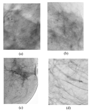
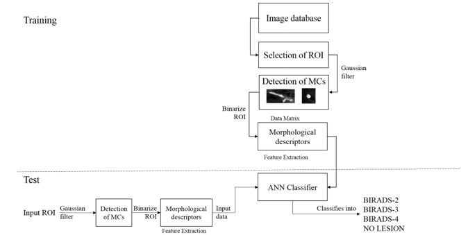
Figure 1 shows examples of samples ROIs used for each category. ROIs were manually obtained from the mammograms.

3.2.  Image Database

Image dataset consists of mammograms of 10 patients for each BIRADS category, 2, 3 and 4. Each patient has 4 mammograms of respective cranial–caudal (CC) view and medio lateral oblique view (MLO) for each breast. For each category 70% of the mammograms were taken for the training stage of the ANN that is mammograms of 7 patients for each category were going to be used to obtain ROIs.

Images format is DICOM (Digital Imaging and Communications in Medicine). DICOM is a standard used worldwide to store, exchange, and transmit medical images. Incorporates standards for imaging modalities such as radiography, ultrasonography, computed tomography, magnetic resonance imaging, and radiation therapy. It also includes protocols for image exchange (e.g., via portable media such as DVDs), image compression, 3-D visualization, image presentation, and results reporting [19].

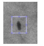
From the selected mammograms ROIs were manually selected, as seen in Figure 2 meaning areas where MCCs were found in the image according to the respective diagnosis given from UNEME-DEDICAM for each patient study. Display resolution of the images is 3540×4740 pixels.

3.3.  Image Enhancement

First a complement of the grayscale ROI image is applied so that black and white pixels are reversed, and MCCs that were originally black pixels are now white pixels, this done in MATLAB. A filter bank script made using MATLAB environment is used to enhance the ROIs previously extracted, said script is a modified version of what research [8] did to detect MCCs. Script consist of applying three filters to the ROI images, Ideal and Gaussian.

The script uses the High Pass Filters which attenuates low frequencies while keeping high frequencies unchanged. Since the high frequencies correspond in the images to sudden changes of density, this type of filters is used, because among other advantages, it offers improvements in the detection of borders in the space domain, since these contain many of these frequencies. It reinforces the contrasts found in the image. This is important as it is possible to detect by sharpening those areas where MCCs are.

Mathematical description of what the high pass Ideal filter does in the script is described by the following transfer function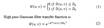

Where D₀ is a specific non negative number which represents the frequency cut-off of the filter and D(u, v) is the distance from point (u, v) to the center of the filter. The script test with different values of D₀.

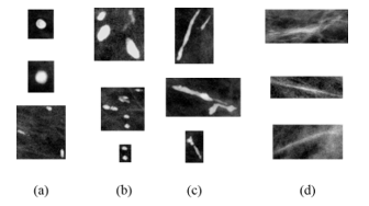
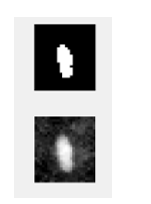
The script gives ROI images in a loop so it is stopped manually to the point where there are around 1000 images and visually select the best ROI image with the MCCs highlighted the best so when the threshold is to be applied the binary mask obtained reflects accurate the region. In this case the configuration to enhance the MCCs was a high pass Gaussian filter with a D₀ value of 0.0021 as seen in Figure 3 for each category.

Once the ROI images are enhanced a threshold is applied and a binary mask is obtained with the region of the MCCs ready to be measured. In Figure 4 there a binary mask of a micro calcification (MC).

3.4.  Data Matrix

To construct a data matrix it is necessary to measure the ROI images that is to measure the region of white pixels in the binary mask, which will give measurements of the MC region. To measure it, it is used regionprops from MATLAB. Region properties selected in this research are:

Area: is the actual scalar number of pixels in the region.

Perimeter: is a scalar that specifies the distance around the boundary of the region.

Centroid: is the center of mass region, in this there are two values, centroid in x and centroid in y.

Equivalent diameter: is the diameter of a circle having the same area with the region.

Euler number: is the number of objects in the region minus the number of holes in those objects.

Major axis length: is the length (in pixels) of the major axis of the ellipse that has the same second moments as the region

Minor axis length: is the length (in pixels) of the minor axis of the ellipse that has the same second moments as the region.

Eccentricity: belongs to the ellipse that has the same second moments as the region, and it is the ratio of the distance between the foci of the ellipse and its major axis length.

Orientation: means the angle (in degrees) between the x-axis and the major axis of the ellipse that has the same second moments as the region [12].

In total 10 features are used to measure MCCs and create a data matrix. Gathering measurements from all the mammograms a 1736 × 10 data matrix. This matrix is standardized, that is take all of the columns of the matrix and standardize / normalize the data so that each data sample exhibits zero mean and unit variance. This means that after this transform, the mean value of any column in this matrix would be 0 and the variance would be 1. This is a very standard method for normalizing values in statistical analysis, machine learning, and computer vision. Following formula describes the calculation of a raw data x into a standard data:

Where u is the mean of the population and σ is the standard deviation of the population [20].

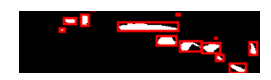
Another property used is Bounding box that returns the smallest rectangle containing the region and it is used to mark the MCs. Figure 5 shows red boxes marking the MCs it is done using the bounding box property.

3.5.  Classification

An ANN is created with the MATLAB toolbox for neural networks to classify the findings in the ROIs in categories BIRADS 2, 3, 4 and No lesion, using the pattern recognition tool.

Neural Network Toolbox™ provides algorithms, functions, and apps to create, train, visualize, and simulate neural networks. You can perform classification, regression, clustering, dimensionality reduction, time-series forecasting, and dynamic system modeling and control [12].

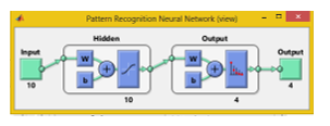
In the Neural Pattern Recognition app data to classify is selected, then a network is created. The network created is a two-layer feed-forward with sigmoid hidden and softmax output neurons, can classify vectors arbitrarily well, given enough neurons in its hidden layer. The network will be trained with

scaled conjugate gradient back propagation, in this research it is used ten neurons in its hidden layers.

Next step is to select the data that is the matrix of 1736 × 10 as input data and as output data is a 1736 × 4 matrix with 1’s indicating to which category the vector belongs. Each column represents a category, being first column the BIRADS 2 and last column No lesion category. If the data vector belongs to category BIRADS 2 then 1 is in that cell in column 1 and the rest is a zero.

In the next stage the Validation and test data, is where data is distributed into Training, Validation and Testing. In here our 1736 sample are randomly divided. For training 70% of the samples, these are presented to the network during training and the network is adjusted to its error. For validation 15% these samples are used to measure network generalization and to halt training when generalization stops improving. And last 15% for testing, these samples have no effect on training and so provide an independent measure of network performance during and after training. Finally our ANN looks as seen in Figure 7

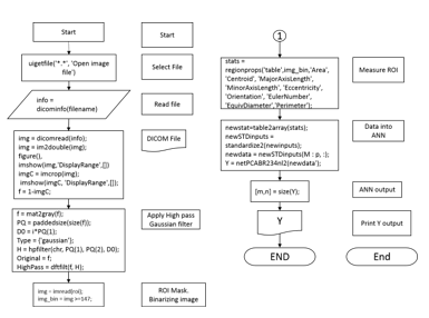
Last part is to measure the performance of the ANN. Tools given are the confusion matrices for training, testing and validation and the plot of the Receiver Operating Characteristic (ROC) curve. The overall methodology used in this research is shown in the diagram in Figure 6. In Figure 8 it is shown the main flow chart of the code used.

4. Experimental results

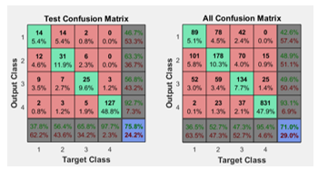
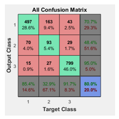
In the confusion matrices the green squares are the correct responses and in the red squares are the incorrect responses. The lower right blue squares illustrate the overall accuracies. In this case a 71% of accuracy in general was obtained, but the Test confusion matrix is the most important as the ANN is classifying samples it didn’t know and a 75.8% was obtained, see Figure 9.

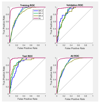
In the plot of the ROC curve the colored lines in each axis represent the ROC curves. The ROC curve is a plot of the true positive rate (sensitivity) versus the false positive rate (1 – specificity) as the threshold is varied. Sensitivity measures the proportion of positives that are correctly identified as such [21] and the false positive rate is the proportion of all negatives that still yield positive test outcomes, i.e., the conditional probability of a positive test result given an event that was not present. A perfect test would show points in the upper-left corner, with 100% sensitivity and 100% specificity [12]. ROC obtained are seen in Figure 10.

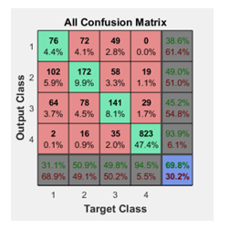
To obtain a better performance of the ANN, it is proposed to apply Principal Component Analysis (PCA) to the data matrix. PCA is a variable reduction technique. It is used when variables are highly correlated. It reduces the number of observed variables to a smaller number of principal components which account for most of the variance of the observed variables. It is a large sample procedure [22]. So this way we expected to discard a region property of the original 10 selected. PCA is applied to the data matrix and outputs 6 descriptors as principal components, those 6 descriptors are area, centroid in x, centroid in y, major axis length, minor axis length and eccentricity. A second network is generated but the overall accuracy gets reduced to a 69.8%, as seen in Figure 11, so using less than the 10 initial descriptors is reducing accuracy so using PCA is discarded.

While experimenting it is notable that the network is having trouble to differentiate the categories BIRADS 2 and 3, as the MCCs in those are very alike in shape, but the difference between them is that the presence of MCCs increases in BIRADS 3. So it is proposed to join this two categories into one and then a new network is generated to train into 3 categories but using the 10 initial descriptors.

Following the last proposal now the ANN is classifying into 3 categories instead of 4, the overall accuracy is 80% meaning that our previous observation of BIRADS 2 and 3 being alike is correct. In Figure 12 it is observed that the ANN performance improved.

In the experimentation stage the hidden neurons were added up to 15 but it did not improved the performance of the ANN, reducing the hidden neurons reduced the percentage of the overall accuracy of the ANN for a very tiny 1%. So modifying the default 10 hidden neurons is discarded.

5. Comparison with state-of-art

As we discussed in the section Previous researches, most of the related researches focus in classifying into two categories, malignant and benignant. As this research focus in the classification method and the system to classify the cancerous findings into BIRADS, our research will be compared against [16] from 2015 and [23] from 2000 which are the more alike as they classify into BIRADS.

First the research conducted by [23] presented an automatic detection and classification of MCCs. A block region growing and K-means clustering-based thresholding is employed to extract the breast region. Then, a blanket method finds and locates the suspicious areas of possible MCCs clusters. The MCCs detection module is developed to automatically extract the MCCs from the ROIs. Among the image processing that are involved in this module are gradient enhancement, contrast enhancement and Gaussian filters. The segmentation of MCCs from the background is done using entropy-based thresholding. Shape cognitron which is based on a neural network-like shape recognition systems is introduced as a classification technique of MCCs. The system achieved as high as 95% classification rate with 93% detection rate [24]. It is important to mention that this particular research has a processing time of 72 seconds as it is completely automatic and it is a more complex methodology, our research is simple, once a ROI is manually selected, goes into a Gaussian filter for denoise, then a binary threshold is applied, regions are measured and finally the data gets classified with a FFNN, all this takes 0.77 seconds of CPU processing time. We obtained an 80% of accuracy, lower against the 95% of [23], it is important to mention they used, 104 cases while we used 120 mammograms. Another difference in methods are that we measure ROIs using morphological descriptors. About the classification technique used they obtained a better accuracy percentage using a neural network-like classifier in our case we are using a more intelligent machine learning technique that is a FFNN that can be tuned every time it is trained and it can learn to be effective. Our research is at disadvantage as it is less accurate, but our methodology is not as complex, and therefore it is faster and barely consume CPU resources.

Next comparing against [16] a computer-aided diagnosis tool for automatic BI-RADS categorization of breast lesions is developed. The user provides parameters such as contour, shape and density and the system gives a suggestion about the BI-RADS classification. Initially, values of malignancy were defined for each image descriptor, according to the BI- RADS standard. When analyzing contour, for example, this method considers the matching of features and linguistic variables. Next, it is created the fuzzy inference system. The generation of membership functions was carried out by the Fuzzy Omega algorithm, which is based on the statistical analysis of the dataset. This algorithm maps the distribution of different classes in a set. Images were analyzed by a group of physicians and the resulting evaluations were submitted to the Fuzzy Omega algorithm. The results were compared, achieving an accuracy of 76.67% for nodules and 83.34%. In this case we are having and ambiguous characterization of the MCCs as it depends of what the user considers is seeing in the mammograms as it is relative to what the user defines as very or little malignancy, as it uses linguistic variables. Contrary to our research where we are actually measuring and obtaining data from the region of the MCC. This data feeds the ANN and helps to obtain an automated classifier.

According to [15] were many classifiers were compared the best is SVM, when classifying binary, next step in our research is explore Multiclass SVM. The advantage of using FFNN is the possibility of classify into more than two categories, therefore achieving to classify into BIRADS. Disadvantage is that our approach is too simple and fails in accuracy, implementing the mesuremnt of MCCs as a cluster could be an improvement for our method as in [23] this approach gave better results than our measuring single MCCs.

6. Conclusions

With the ROC plot it is observed that the best category to classify was the No lesion, from the other 3, meaning that our ANN is accurately discerning from a non-lesion and a lesion or MC. Also the initial 10 descriptors are the better choice and reducing them did not gave a better performance so in future works more descriptors will be added. We are already experimenting with Multiclass SVM as seen in surveys that SVM is better than ANN but as a binary classifier, in our case we’ll classify into more categories.

Acknowledgment

We wish to thank Universidad Autónoma de Querétaro (UAQ) for the academic support for this project research and CONACyT, México for the financial support.

1. E. D. Avalos-Rivera and A. D. J. Pastrana-Palma, “Classifying microcalcifications on digital mammography using morphological descriptors and artificial neural network,” IEEE Congr. Argentino Ciencias la Informática y Desarro. Investig., 2016.
2. H. D. Cheng, X. Cai, X. Chen, L. Hu, and X. Lou, “Computer-aided detection and classification of microcalcifications in mammograms: a survey,” Pattern Recognit., vol. 36, no. 12, pp. 2967–2991, Dec. 2003.
3. W. Jian, X. Sun, and S. Luo, “Computer-aided diagnosis of breast microcalcifications based on dual-tree complex wavelet transform.,” Biomed. Eng. Online, vol. 11, p. 96, 2012.
4. R. Audelo-Valverde and A. Pastrana-Palma, “Clasificación de Microcalcificaciones utilizando Descriptores Morfológicos,” Universidad Autonoma de Queretaro, 2014.
5. A. Tirtajaya and D. D. Santika, “Classification of Microcalcification Using Dual-Tree Complex Wavelet Transform and Support Vector Machine,” in 2010 Second International Conference on Advances in Computing, Control, and Telecommunication Technologies, 2010, pp. 164–166.
6. P. Görgel, A. Sertbas, and O. N. Uçan, “Computer-aided classification of breast masses in mammogram images based on spherical wavelet transform and support vector machines,” Expert Syst., vol. 32, no. 1, pp. 155–164, 2015.
7. B. Joseph, B. Ramachandran, and P. Muthukrishnan, “Intelligent Detection and Classification of Microcalcification in Compressed Mammogram Image,” Image Anal. Stereol., no. 1997, pp. 183–198, 2015.
8. L. A. Salazar-Licea, J. C. Pedraza-Ortega, and A. Pastrana-Palma, “Algoritmos de procesamiento digital de imagenes para la deteccion de microcalcificaciones a partir del analisis de mamografias,” Universidad Autonoma de Queretaro, 2015.
9. A. Shirazinodeh, H. A. Noubari, H. Rabbani, and A. M. Dehnavi, “Detection and classification of Breast Cancer in Wavelet Sub – bands of Fractal Segmented Cancerous Zones,” vol. 5, no. 3, 2015.
10. P. Ricci, A. Cruz, M. Rodríguez, H. Sepúlveda, I. Galleguillos, F. Rojas, V. Peña, R. Carvajal, M. Bravo, R. Castillo, and C. Núñez, “Trabajos Originales MICROCALCIFICACIONES BIRADS 4: EXPERIENCIA DE 12 AÑOS,” Rev Chil Obs. Ginecol, vol. 71, no. 6, pp. 388–393, 2006.
11. R.-A. Gibran and A. Pastrana-Palma, “Implementación de un Diagnóstico Asistido por Computadora para la Detección de Microcalcificaciones en Mamografías,” Universidad Autonoma de Queretaro, 2014.
12. MATLAB R2016a Product Help. .
13. C. J. V. Y. Jiang, R. M. Nishikawa, E. E.Wolverton, C. E. Metz, M. L. Giger, R. A. Schmidt, “Malignant and benign clustered micro- calcifications: automated feature analysis and classification,” Radiology, vol. 198, pp. 671–678, 1996.
14. D. K. Jiang Y, Nishikawa RM, Schmidt RA, Metz CE, Giger ML, “Improving breast cancer diagnosis with computer-aided diagnosis,” Acad. Radiol., vol. 6, pp. 22–33, 1999.
15. R. M. Nishikawa, “A study on several Machine-learning methods for classification of Malignant and benign clustered microcalcifications,” IEEE Trans. Med. Imaging, vol. 24, no. 3, pp. 371–380, Mar. 2005.
16. G. H. B. Miranda and J. C. Felipe, “Computer-aided diagnosis system based on fuzzy logic for breast cancer categorization,” Comput. Biol. Med., vol. 64, pp. 334–346, 2015.
17. F. P. Kestelman, G. A. De Souza, L. C. Thuler, G. Martins, V. Aguilera, R. De Freitas, and E. D. O. Canella, “BREAST IMAGING REPORTING AND DATA SYSTEM – BI-RADS ®: POSITIVE PREDICTIVE VALUE OF CATEGORIES 3 , 4 AND 5 . A SYSTEMATIC LITERATURE REVIEW *,” vol. 40, no. 3, pp. 173–177, 2007.
18. American College of Radiology, Breast Imaging Reporting and Data System Atlas (BI-RADS Atlas). Reston (VA), 2003.
19. C. E. Kahn, J. A. Carrino, M. J. Flynn, D. J. Peck, and S. C. Horii, “DICOM and Radiology: Past, Present, and Future,” J. Am. Coll. Radiol., vol. 4, no. 9, pp. 652–657, Sep. 2007.
20. E. Kreyszig, Advanced Engineering Mathematics, 4th ed. 1979.
21. “Detector Performance Analysis Using ROC Curves – MATLAB & Simulink Example.” [Online]. Available: www.mathworks.com.
22. P. M. Jain and V. . . Shandliya, “A survey paper on comparative study between Principal Component Analysis ( PCA ) and Exploratory Factor Analysis ( EFA ),” Int. J. Comput. Sci. Appl., vol. 6, no. 2, pp. 373–375, 2013.
23. S. Lee, C. Lo, C. Wang, P. Chung, C. Chang, C. Yang, and P. Hsu, “A computer-aided design mammography screening system for detection and classification of microcalcifications.,” Int. J. Med. Inform., vol. 60, no. 1, pp. 29–57, 2000.
24. N. Yusof, N. Ashidi, M. Isa, H. Amylia, and M. Sakim, “Computer-Aided Detection and Diagnosis for Microcalcifications in Mammogram: A Review,” vol. 7, no. 6, pp. 202–208, 2007.

(Click to view)

(Click to view)