Use of machine learning techniques in the prediction of credit recovery

1 Introduction

This paper is an extension of the work originally presented at the International Conference on Machine Learning and Application (ICMLA 2016) [1], which presented the first results of a Brazilian bank research to reduce its losses with defaulting clients. That study covered only a sample of 22.764 transactions, representing a homogeneous group of bank customers. We extend our previous work by adding all operations from individual costumers which were in arrears in July 2016.

The Figure 1 shows that there was a slight decrease in the number of debtors in June 2016, but increased again in the following months.

The Bank had nearly 54 million active credit agreements with individuals at the end of July 2016. Of this amount, approximately 8.6 million were delayed for 15 days or more, accounting for 15.9% of the contracts. These delinquent contracts amounted to more than R$20.8 billion (US$6.4 billion in July 2016), accounting for approximately 5.8% of the Bank’s individuals loan portfolio, an increase of 1.2 percentage points over December 2014. That is, in 21 months the financial volume of overdue loans contracted by individuals increased by 26%.

The Brazilian Central Bank (BACEN) regulation requires financial institutions to classify their credit operations and perform a Provision for Doubtful Accounts (PDA), according to a risk classification. The main criteria for the classification is the number of days in arrears of each individual credit agreement.

The Table 1 shows the days-in-delay ranges considered to determine a risk classification and therefore the minimum percentage PDA that financial institutions must reserve. As an operation increases the number of days in arrears, there is a non-linear increase of PDA, which may allocate 100% of the outstanding balance of the contract. For example, an operation with a debit balance of R$ 1,000, with 15 days in arrears, must reserve a minimum provision of R$ 10. The amount of the provision may reach R$ 1,000 if the arrear reach 180 days.

Table 1: Days in arrears x Provision

Days in arrears	Minimum Risk	PDA %
15-30	B	1
31-60	C	3
61-90	D	10
91-120	E	30
121-150	F	50
151-180	G	70
over 180	H	100

At the time of the credit granting, financial institutions assume the credit risk and make the corresponding provisions in accordance with the current Central Bank regulation. Acting in this way, in a possible default of the customer, the financial institution and the stability of the financial system will be protected. However, as a customer delays its operations, the natural reaction of financial institutions is to restrict credit to them, increasing the chances of these

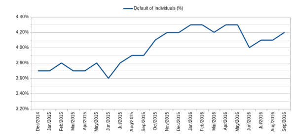Figure 1: Default of individuals.

customer’s evasion to other institutions, since they will not be able to carry out new credit operations with the original institution.

With the increase in delinquency, a mobilization of account managers of the bank began in order to mitigate the evasion of its clients by approaching the customer in arrear and proposing alternatives that could fix the delayed payments. Hence, solving the default situation and the possible loss of the customer of its portfolio, as well as reducing the financial amount allocated to (PDA).

Provided that the selection of the clients is a time and resource consuming task, the main objective of this study was to apply machine learning techniques to predict the recovery probability of credit transactions, providing a list of delinquent clients with the greatest potential for regularization of their operations.

Models were developed using Generalized Linear Models (GLM), Gradient Boosted Methods (GBM), Distributed Random Forest (DRF) and Deep Learning (DL)^[1] . The models were compared using the recall indicator, which will be explained on section 3. The models were developed using the R language and H2O machine learning platform, considering its parallel processing capabilities. Further details on section 3. ²

This paper is organized as follows: Section 2 presents the credit scoring state of the art. Section 3 presents the methodology used in this study. Section 4 presents the modeling and evaluation of the generated models for each method. Section 5 presents the conclusion and future works.

2 State of the Art

The default numbers observed in Brazil, from December 2014 to September 2016, indicate that financial institutions need a tool to support their credit granting decisions. Although there are several studies to identify the customer credit risk, qualifying them as good or bad payers, helping to make a decision to grant credit, there is few research studying the credit recovery, when the delinquency occurs. [2]

In [3], the author conducted a study evaluating 41 publications on the award of credit since 2006, all of them using classifiers to categorize customers as good or bad payers. Those works were organized into three categories of classifiers: individuals; homogeneous ensemble; and heterogeneous ensemble classifiers. Most of the algorithms used were implemented through logistic regression and decision trees, with their use of boosting, bagging and forest variants.

The Table 2 lists the eight datasets that were used in [3] to verify the performance of each of the 41 models proposed, evaluating them from the standpoint of 6 indicators: Area Under the Receiver Operating Curve (AUC), percentage correctly classified (PCC), partial Gini index, H-measure, Brier Score (BS) and Kolmogorov-Smirnov (KS).

Table 2: Datasets used in [3].

Name	Samples	Features	Debtors %
AC	690	14	44.5
GC	1000	20	30.0
Th02	1225	17	26.4
Bene 1	3123	27	66.7
Bene 2	7190	28	30.0
UK	30000	14	4.0
PAK	50000	37	26.1
GMC	150000	12	6.7

In [4], the author presents AUC as an indicator that represent how well classified were the data, independent of its distribution or misclassification costs. PCC is an overall accuracy measure that indicates the percentage of outcomes that were correctly classified.[5]

A score was assigned to each algorithm, referring to the classification received in the comparison between them within the same performance measure . For example, the algorithm K-means was in 12th place considering the AUC indicator, while the KNN was in 29th place. Thus, the scores attributed to them were 12 and 29, respectively. Then, the algorithms were ordered by the average of all metrics, where the 1st place were the algorithm that obtained the lowest score.

The heterogeneous multi-classifiers presented a better performance, although the performance between the three categories was very similar.

The Table 3 presents the results of the benchmark, indicating that the HCES-Bag algorithm obtained the highest AUC result, while the AVG-W and Gasen algorithms reached 80.7% of the PCC.

	Algorithm	AUC	PCC
	HCES-Bag	0.932	80.2
Heterogeneous Ensemble	AVG W	0.931	80.7
	GASEN	0.931	80.7
	RF	0.931	78.9
Homogeneous Ensemble	BagNN	0.927	80.2
	Boost	0.93	77.2
	LR	0.931	70.84
Individual	LDA	0.929	78.4
	SVM-Rbf	0.925	79.9

Table 3: State of Art – Models Comparison – Adapted from [3]

3 Methodology and Infrastructure Setup

This section presents the methodology used in this study, which was segmented in stages according to the phases proposed by CRISP-DM [6]. The result of each phase is described in the next Section.

Training model environment – The models were trained on the H2O.ai platform, in a cluster formed by 5 virtual machines on the same subnet and with the same configuration. Their operating system was Red Hat Enterprise Linux 6.8 64 bits, with 34 cores and 80

GB of RAM. It were used H2O.ai version 3.10.4.5 and R version 3.3.0. It were allocated 44 GB of RAM and all cores of each machine, reaching a total of 170 cores and 220 GB of RAM.

The training dataset consisted of about 40 million copies, requiring a robust platform to be made available for the processing of this data.

The Figure 2 shows the CPU meter of the H2O.ai cluster in action at the moment of the training models. It shows the percentage of use of the processors of each machine, identified by the final number of its IP address (174 to 178) and the port number where the service was running (54321). The intensive use of the 170 available cores shown in the Figure 2 reinforces the need for a robust platform.

Each vertical bar represents 1 core and the colors represent the type of process executed: idle time (blue), user time (green) and system time (red).

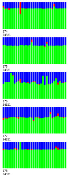Figure 2: Cluster H2O in action

4 Results

In this sections, the results of the CRISP-DM phases are detailed: Data Understanding, Data preparation, Modeling, Evaluation and Implementation.

4.1       Data Understanding

The dataset was obtained by the extraction of information from legacy systems and customers relationship data marts. It has information about customers accounting,demographic and financial data. The dataset had 28 features and 1 label that indicates the recovery of the respective credit operation. The

Tables 4 and 5 present these 28 characteristics organized by categorical and numerical features.

Table 4: Numeric features

Features	Description
V1	Number of days of delinquency.
V2	Number of days remaining for the end of the contract.
V3	Contract value.
V4	Amount of the outstanding balance.
V5	Amount PDA provisioned for the contract.
V6	Percentage loss expected for the contract.
V7	Quantity of products owned by the customer.
V8	Time of customer relationship with the Bank.
V9	Customer age.
V10	Customer income.
V11	Customer total contribution margin amount.
V12	Value of Gross Domestic Product per capita

Table 5: Categorical features

Features	Description
VC1	Customer portfolio type.
VC2	Customer behavioral segment.
VC3	Product.
VC4	Product modality.
VC5	Structured operation indicator.
VC6	Management level that approved the operation.
VC7	Transaction risk credit.
VC8	Range of past delays.
VC9	PDA lock indicator.
VC10	Customer               relationship                with        the bank.
VC11	Client instruction level.
VC12	Customer gender.
VC13	Nature of customer occupation.
VC14	Customer registration status.
VC15	Customer’s age group.
VC16	Age group of relationship time.

For the data understanding, the analysis began in July 2016 containing all credit operations contracts, regardless of the contracted product, with more than 14 days in arrears. In addition, transactions with the highest risk were considered as already lost contracts by our business specialists and removed from our dataset.

For definition of the label, the delay reduction indicator, the following operation was performed, considering that the data of the delayed operations were used in July 2016:

• Delay Reduction Indicator = 1, for all transactions that showed a reduction in the number of days overdue in the subsequent month, that is, in August 2016, or that their debit balances have been reduced.
• Delay Reduction Indicator = 0, otherwise, that is, presenting a delay or debit balance in August 2016 equivalent to or greater than that observed in July 2016.

The Table 6 presents the summary of transactions in the month of July 2016, which resulted in a base with 4,514,029 contracts. Of this total, only 271,193 (6.01%) were recovered.

Table 6: Dataset July 2016

Not recovered	Recovered
4,242,836	271,193
93.99%	6.01%
Samples	4,514,029

The bank has several strategies for credit recovery, according to the customer profile and the category of the credit operation, grouping them with distinct trading rules. Existing segments are divided into massive and individual strategies. Massive strategies are implemented for segments that have a known behavior pattern, whereas individual strategies cover operations that have atypical or special characteristics which require a case-by-case analysis to perform a collection and recovery.

Based on this information, the dataset was splitted into segments compatible with the institution’s recovery strategies, grouping similar products and customer segments with characteristics in common removing from the study the segments that have an individualized trading strategy. The Table 7 lists the 11 segments that will be worked on in this study, in addition to the Individualized Strategy segment, which was removed from the study.

4.2       Data Preparation

In this study, the analysis were performed only in the first 3 segments, Mortgage Loan I, II and III. The remaining segments are in the final analysis phase and will be presented at a later time.

Then, the data preparation was started, analyzing each one of the segments, preparing the data sets for the modeling phase.

The Tables 8, 10 and 12 present the summary of descriptive analysis of the numerical features of segments Mortgage Loan I, II and III, respectively. In these tables the data of quartiles and Kendall’s Tau [7] of each feature are presented.

The Tables 9, 11 and 13 present the summary of the descriptive analysis of the categorical variables, listing the Kendall’s Tau and the number of levels of each feature.

Table 7: Credit Operations Segments Segment Credit Recovered Samples No Yes Qty % Qty % Mortgage Loan I 41,398 70.45 17,365 29.55 58,763 Mortgage Loan II 400 73.94 141 26.06 541 Mortgage Loan III 3,537 78.11 991 21.89 4,528 Vehicle Financing I 12,115 87.90 1,667 12.10 13,782 Vehicle Financing II 32,357 86.63 4,993 13.37 37,350 Agribusiness 258,618 98.84 3,021 1.16 261,639 Social Business 137,474 93.53 9,504 6.47 146,978 Credit Card I 17,124 98.92 187 1.08 17,311 Credit Card II 454,864 98.56 6,661 1.44 461,525 Other Operations Income I 186,572 96.53 6,714 3.47 193,286 Other Operations Income II 2,668,890 92.96 201,977 7.04 2,870,867 Individualized Strategy 429,487 95.98 17,972 4.02 447,459 .. Table 8: Mortgage Loan I – Numerical Features Feature Min 1QT Median Avg 3QT Max Kendall’s Tau V1 15 20 51 87.43 112 624 -0.29 V2 0 10,180 10,420 10,290 10,670 11,620 -0.03 V3 0 0.1 0.13 0.17 0.27 0.67 -0.02 V4 0 1 2 3.94 5 26 0.06 V5 17 25 29 31.28 36 73 0.03 V6 1 3 4 4.45 5 37 0.08 V7 14,790 74,400 87,460 86,270 97,470 164,800 0.01 V8 -124,400 -390.8 156.7 -1,397 256.3 183,400 0.38 V9 0 1,349 3,221 3,712 5,525 46,040 0.04 V10 0 888.1 2,670 19,090 20,960 173,700 -0.17 V11 0 1,586 1,700 1,877 2,000 20,000 0.03 V12 0.68 74,920 88,720 87,250 99,510 173,500 0.00

4.3      Modeling

For each dataset, 4 predictive models were elaborated, using the H2O platform integrated to the R, using the algorithms Generalized Linear Models (GLM), Gradient Boosting Method (GBM), Random Forest (DRF) and Deep Learning (DL). The first three algorithms were chosen because they represent the techniques most used in the calculation of credit risk, which performs a classification task very similar in [8]. The algorithm DL was used to verify its behavior in a knowledge area not yet explored, but with expectation of good suitability due to the use of a great amount of

variables. [9]

The datasets of the Mortgage Loan I and III segments were splitted into 3 parts: 70% for training, 20% for validation and 10% for testing. Due to the small number of observations in the Mortgage Loan II, this dataset was splitted only in training and validation in a proportion of 80% and 20%, respectively. The next subsections present the evaluation results for each segment.

4.3.1       Mortgage Loan I

• GLM – This algorithm obtained an AUC = 0.7774755 and a PCC of 66.53%, as shown in the Figure 3 and in the Table 14

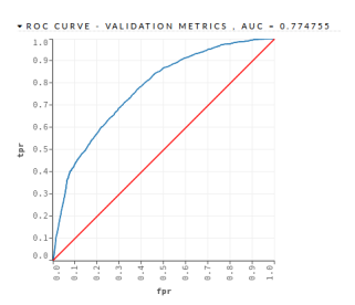Figure 3: Mortgage Loan I – GLM – Validation Dataset

Table 9: Mortgage Loan I – Categorical Features Feature Kendall’s Tau Number of levels VC1 0.23 6 VC2 0.02 5 VC3 -0.09 3 VC4 -0.21 9 VC5 0.03 12 VC6 0.06 7 VC7 -0.01 2 VC8 0.03 5 VC9 -0.04 16 VC10 0.00 4 VC11 0.05 8 VC13 -0.21 9 VC14 0.01 4 VC15 -0.02 18 VC16 0.00 2 Table 10: Mortgage Loan II – Numerical Features Feature Min 1QT Median Avg 3QT Max Kendall’s Tau V1 15 21 48 89 113 507 -0.15 V2 0 1,626 2,928 3,037 4,076 6,776 -0.14 V3 0 0 0 0 0 1 0.09 V4 2 6 6 10 13 31 0.03 V5 30 42 48 49 55 85 0.02 V6 1 4 6 7 9 36 -0.04 V7 4,400 28,000 45,000 59,560 70,560 240,000 -0.05 V8 -31,770 -148 91 -650 371 25,070 0.30 V9 0 4,990 6,190 6,663 9,099 15,260 0.08 V10 0 173 650 8,744 10,230 116,000 -0.20 V11 0 1,598 2,965 5,082 5,553 128,900 -0.11 V12 0 9,316 20,500 36,670 47,120 215,200 -0.14

• DRF – This algorithm was implemented with 500 trees and a maximum depth of 7. The DRF algorithm obtained an AUC = 0.880589 and a PCC = 75.85%, as shown in the Figure 4 and in the Table 14

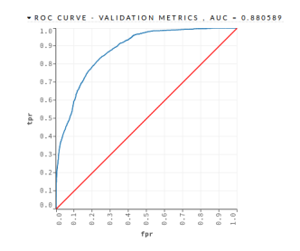Figure 4: Mortgage Loan I – DRF – Validation Dataset

AUC

• DL – Deep Learning This algorithm was implemented with 2 hidden layers with 200 neurons each one. The DRF algorithm obtained an AUC = 0.898203 and a PCC = 79.22%, as shown in the Figure 5 and in the Table 14.

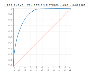Figure 5: Mortgage Loan I – DL – Validation Dataset

Table 11: Mortgage Loan II – Categorical Features Features Kendall’s Tau Number of levels VC1 0.11 4 VC2 0.13 3 VC4 -0.19 8 VC5 0.01 10 VC6 0.03 6 VC7 -0.04 2 VC8 0.10 5 VC9 0.06 10 VC11 -0.15 5 VC13 -0.19 8 VC14 0.10 4 VC15 -0.06 13 Table 12: Mortgage Loan III – Numerical Features Feature Min 1QT Median Avg 3QT Max Kendall’s Tau V1 15 30 81 131 181 511 -0.31 V2 0 4,876 7,530 6,616 8,203 10,910 -0.01 V3 0.00 0.02 0.05 0.06 0.07 0 0.00 V4 0 5 9 11 15 54 -0.02 V5 20 35 43 44 52 78 -0.06 V6 2 6 8 10 11 71 0.05 V7 20,000 100,000 142,500 188,700 213,800 3,000,000 -0.07 V8 -257,600.00 -5,476.00 -930.00 -9,087.00 257.70 199,600 0.36 V9 0 2,769 4,660 4,968 6,485 46,040 0.01 V10 0 3,317 14,200 51,540 53,470 1,212,000 -0.20 V11 0 2,280 5,542 10,700 11,130 337,600 -0.01 V12 250 88,900 134,500 177,500 203,200 3,084,000 -0.08

• GBM – This algorithm was implemented with 500 trees and a maximum depth of 7. The GBM algorithm obtained an AUC = 0.988574 and a PCC = 93.90%, as shown in the Figure 6 and in the Table 14

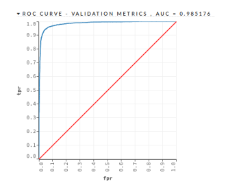Figure 6: Mortgage Loan I – GBM – Validation Base

AUC

4.3.2        Mortgage Loan II

Because of the small number of records, this dataset was splitted only in training and testing, in the ratio of 80:20, and validation was performed through cross validation with 10 folds.

• GLM – This algorithm obtained an AUC = 0.848474 and a PCC = 65.51%, as shown in the Figure 7 and in the Table 15.

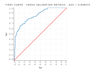Figure 7: Mortgage Loan II – GLM – Validation Dataset

Table 13: Mortgage Loan III – Categorical Features

Feature	Kendall’s Tau	Number of levels
VC1	0.16	6
VC2	0.00	4
VC3	-0.24	2
VC4	-0.21	33
VC5	-0.06	12
VC6	-0.02	7
VC7	-0.03	2
VC8	0.00	5
VC9	-0.02	16
VC10	-0.10	5
VC11	0.03	7
VC12	0.00	2
VC13	-0.21	9
VC14	0.00	5
VC15	-0.04	17
VC16	0.17	2

Table 14: Mortgage Loan I – Confusion Matrix

Algorithm		0	1	Err %	PCC
GLM	0	5003	3050	37.87
	1	776	2603	22.96
	Total	5779	5653	33.46	66.52
DRF	0	6638	1415	17.57
	1	816	2563	24.14
	Total	7454	3978	19.51	75.85
DL	0	6290	1763	21.89
	1	517	2862	15.39
	Total	6897	4625	19.94	79.22
GBM	0	7770	283	3.51
	1	238	3141	7.04
	Total	8008	3424	4.55	93.90

Algorithm		0	1	Err %	PCC
GLM	0	270	35	11.47
	1	40	76	34.48
	Total	310	111	17.81	65.51
DRF	0	302	3	0.98
	1	17	99	14.65
	Total	319	102	4.75	85.34
DL	0	297	8	2.62
	1	10	106	8.62
	Total	307	114	4.27	91.37
GBM	0	301	4	1.31
	1	16	100	13.79
	Total	317	104	4.75	86.20

         Table 15: Mortgage II – Confusion Matrix

Figure 8: Mortgage Loan II – DRF – Validation Dataset

AUC

• DRF – This algorithm was implemented with 500 trees and a maximum depth of 7. The DRF algorithm obtained an AUC = 0.977982 and a • DL – This algorithm was implemented with 2 PCC = 93.10%, as shown in the Figure 8 and in hidden layers with 200 neurons each one. The the Table 15 DRF algorithm obtained an AUC = 0.956868

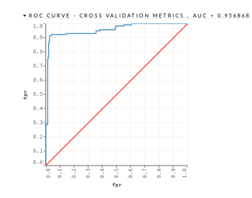Figure 9: Mortgage Loan II – DL – Validation Dataset AUC

• GBM – This algorithm was implemented with 500 trees and a maximum depth of 7. The GBM algorithm obtained an AUC = 0.972640 and a PCC = 86.20%, as shown in the Figure 10 and in the Table 15

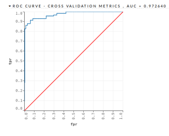Figure 10: Mortgage Loan II – GBM – Validation

Dataset AUC

4.3.3        Mortgage Loan III

• DRF – This algorithm was implemented with 500 trees and a maximum depth of 7. The DRF algorithm obtained an AUC = 0.950718 and a PCC = 83.51%, as shown in the Figure 11 and in the Table 16
• DL – This algorithm was implemented with 2 hidden layers with 200 neurons each one. The DRF algorithm obtained an AUC = 0.939082 and a PCC = 78.20%, as shown in the Figure 12 and in the Table 16.

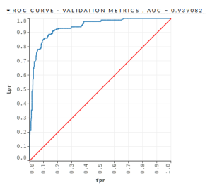Figure 12: Mortgage Loan III – DL – Validation Dataset

AUC

• GBM – This algorithm was implemented with 500 trees and a maximum depth of 7. The GBM algorithm obtained an AUC = 0.955728 and a PCC = 98.93%, as shown in the Figure 13 and in the Table 16

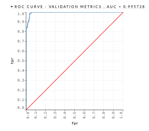Figure 13: Mortgage Loan III – GBM – Validation Dataset AUC

• GLM – This algorithm obtained an AUC =

0.814560 and a PCC = 60.10%, as shown in the Figure 14 and in the Table 16

Table 16: Mortgage Loan III – Confusion Matrix

Algorithm	0	1	Err %	PCC
GLM	601	95	13.64
	75	113	39.89
	676	208	19.23	60.10
DRF	640	56	8.04
	31	157	16.48
	671	213	9.84	83.51
DL	656	40	5.74
	41	147	21.80
	697	187	9.16	78.20
GBM	670	26	3.73
	2	186	1.06
	672	212	3.16	98.93

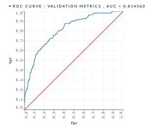Figure 14: Mortgage Loan III – GLM – Validation

Dataset AUC

5 Conclusion

The main objective of this study was to apply machine learning techniques to predict the probability of recovery of credit transactions, providing a list of defaulting clients with greater potential for regularization of their operations.

Studies were carried out on 3 segments of credit operations, which have different recovery strategies, the Mortgage Loan segments I, II and III. With the machine learning, it was possible to elaborate predictive models with great contribution to assist the Managers in the approach to their clients with operations in arrears.

Mortgage Loan I – The model with the highest recall was obtained with the GBM algorithm. In a total of 11,342 contracts in default, there were 3,424 contracts recovered. The model was able to correctly predict 3,141 contracts, reaching a recall of 92.86%. Using the prioritization list generated by the model, the work of Bank Managers would be more assertive. In addition, the model correctly predicted 7,770 (97.02%) contracts, out of 8,008 contracts that would not be recovered.

Mortgage Loan II – The model with the highest recall was obtained with the DL algorithm. In a total of 421 delinquent contracts, there were 116 contracts recovered. The model was able to correctly predict 106 contracts, reaching a recall of 94.38%. In addition, the model correctly predicted 297 (96.74%) contracts out of 307 contracts that would not be recovered.

Mortgage Loan III – The model with the highest recall was obtained with the GBM algorithm. In a total of 884 delinquent contracts, there were 212 contracts recovered. The model was able to accurately predict 186 contracts, reaching a recall of 98.94%. In addition, the model correctly predicted 670 (99.70%) contracts out of 672 contracts that would not be recovered.

The predictive models obtained from the analysis of the first three segments, out of a total of 11, have already shown a potential great benefit to the bank, effectively assisting its customers with delayed operations and avoiding unnecessary efforts in attempts in attempts of negotiation in contracts with low probability of recovering.

5.1      Future Works

The results obtained so far strengthen initiatives for the development of predictive models using machine learning techniques in the Bank studied.

With the increase in the efficiency of credit recovery, the Bank will benefit from the reduction in Allowance for Loan Losses (PDA), directly promoting positive results, with the reversal of provisions already made.

Thus, the study will be expanded to the 8 segments that have not yet been modeled, increasing the use of models obtained through machine learning techniques in credit recovery. In addition, the models al-

1. Rogerio G. Lopes, Rommel N. Carvalho, Marcelo Ladeira, and Ricardo S. Carvalho. Predicting Recovery of Credit Operations on a Brazilian Bank. pages 780–784. IEEE, December 2016.
2. Sung Ho Ha. Behavioral assessment of recoverable credit of retailer’s customers. Inf. Sci., 180(19):3703–3717, October 2010.
3. Stefan Lessmann, Bart Baesens, Hsin-Vonn Seow, and Lyn C. Thomas. Benchmarking state-of-the-art classification algorithms for credit scoring: An update of research. European Journal of Operational Research, 247(1):124–136, 2015.
4. Wouter Verbeke, Karel Dejaeger, David Martens, Joon Hur, and Bart Baesens. New insights into churn prediction in the telecommunication sector: A profit driven data mining approach. European Journal of Operational Research, 218(1):211 – 229, 2012.
5. Karel Dejaeger, Frank Goethals, Antonio Giangreco, Lapo Mola, and Bart Baesens. Gaining insight into student satisfaction using comprehensible data mining techniques. European Journal of Operational Research, 218(2):548 – 562, 2012.
6. Pete Chapman, Julian Clinton, Randy Kerber, Thomas Khabaza, Thomas Reinartz, Colin Shearer, and Rudiger Wirth. Crisp-dm 1.0 step-by-step data mining guide. Technical report, The CRISP-DM consortium, August 2000.
7. Stephan Arndt, Carolyn Turvey, and Nancy C Andreasen. Cor-relating and predicting psychiatric symptom ratings: Spearmans r versus kendalls tau correlation. Journal of psychiatric research, 33(2):97–104, 1999.
8. Bart Baesens, Tony Van Gestel, Stijn Viaene, Maria Stepanova, Johan Suykens, and Jan Vanthienen. Benchmarking state-of-the-art classification algorithms for credit scoring. Journal of the operational research society, 54(6):627–635, 2003.
9. Yann LeCun, Yoshua Bengio, and Geoffrey Hinton. Deep learning. Nature, 521(7553):436–444, 2015.

(Click to view).

(Click to view).