1. Introduction

The extracted output power from the photovoltaic (PV) system is affected by the climate conditions represented by a solar irradiation (G) and a temperature (T). Hence, an effective maximum power point tracking technique is required improve the efficiency of the overall PV system.

In the last years, many MPPT techniques have been proposed to track the MPP of the PV module [1–6]. In [1], the FLC based MPPT is proposed to track the MPP at standard technical condition (STC) and variable resistive load. Where, the change in duty cycle (ΔD) was used as an FLC’s output to adjust the duty cycle (D) of the DC-DC converter, in order to meet the load matching between the PV module and the connected resistive load.

This work is an extension of work originally presented in 2016 International Conference on Applied and Theoretical Electricity (ICATE) [1]. In this paper, the efficiency of FLC-based MPPT for the PV system is examined under variable climate conditions (irradiation and temperature) and variable values of connected resistive load. The utilized PV system includes a BP SX150S PV module, buck-boost DC-DC converter, MPPT controller, and resistive load (R_L). The circuit diagram of the PV system is shown in Figure 1.

The rest of this paper is arranged as follows: Section 2 explains the basic modeling of the utilized PV module. Section 3 tackles the MPPT control and the mechanism of load matching through the DC-DC converter. Section 4 describes the details of considered MPPT algorithms: conventional perturb and observe (P&O) and the proposed FLC. Simulation and comparison results obtained by using Matlab software are presented in Section 5. Finally, conclusions of the work are revealed in Section 6.

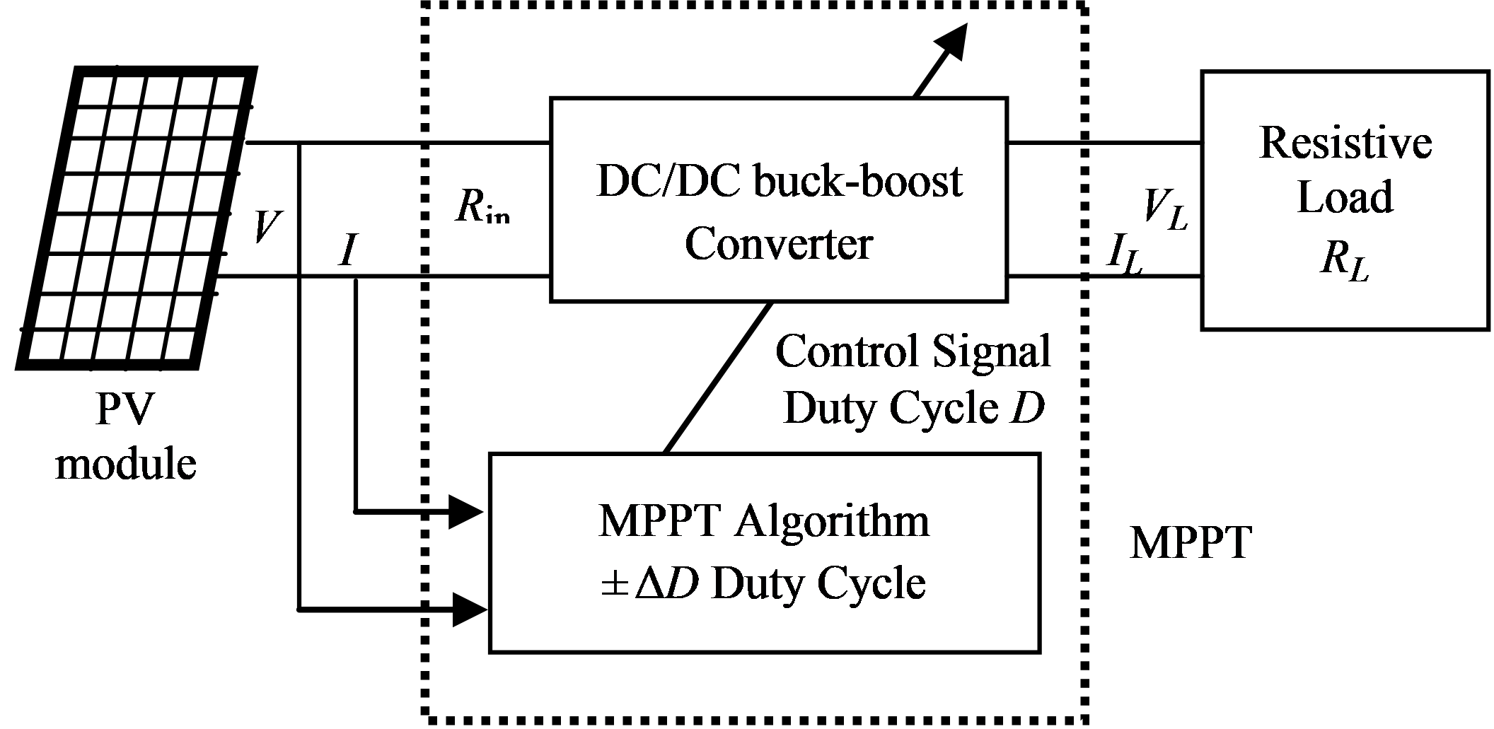Figure 1. The PV system with MPPT control.

2.       Modeling of the PV Module

In this paper, a single-diode equivalent circuit model is used. This model consists of two resistances (series R_s and parallel R_sh) as depicted in Figure 2 [7].

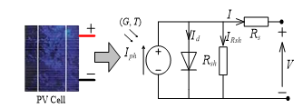Figure 2. The equivalent circuit of the PV model.

According to the Kirchhoff’s law, the characteristic equation of the PV model can be expressed by [8]:

By developing the terms of I_d and I_Rsh, the PV current can be written as,

Where I_ph is the light current that is equal to short-circuit current I_sc. I_d and I_Rsh are the parallel currents through the diode and parallel resistance R_sh, respectively. I_o is the cell’s reverse saturation current, also known as the “dark current”, q is the electron charge (1.602×10^-19 C), n is the diode ideality factor of a value is between 1 and 2, K is the Boltzmann’s constant (1.381×10^-23 J/K), T is the PV cell temperature (K), and N_s is the number of series-connected solar cells to organize the utilized PV module [1,8,9]. In this paper, the BP SX150S PV of N_s =72 cells is utilized to produce a peak power output of 150 W at standard technical condition (STC). Under STC, the cell temperature T_r is 298 ^oK which equivalent to 25 ^oC and the solar irradiation G_r is 1000 W/m² at air mass (AM=1.5). Table 1 illustrates the utilized PV module’s electric parameters [10].

Table 1. Electrical parameters of BP SX150S PV module

Parameter	Value
Maximum Power (Pmax)	150 W
Voltage at Pmax (Vmpp)	34.5 V
Current at Pmax (Impp)	4.35 A
Short-circuit current (Isc)	4.75 A
Open-circuit voltage (Voc)	43.5 V
Temperature coefficient of Isc	(0.065 ± 0.015) %/ oC
Temperature coefficient of Voc	– (160 ± 20) mV/ oC

The reverse saturation current (I_o) is dependent on the temperature (T) and can be expressed by:

Where E_g is the band-gap energy of the semiconductor used in the cell.

To determine the module’s open-circuit voltage (V_oc), we set (I=0 and V=V_oc) and assume R_sh= ∞ in (2), which results,

The PV module’s short-circuit current (I_sc) depends on the cell temperature (T) and solar irradiation (G) as,

Where α is the short circuit current temperature coefficient.

The PV module’s maximum power point (MPP) is the point at which the peak product of V and I is obtained, hence V=V_mpp, I=I_mpp, and P=P_max at MPP. This point changes with the variation of climate conditions as shown in Figure 3 and Figure 4. It can be seen that the current and power of the PV module increase linearly as irradiation increases, while the voltage approximately unchanged as shown in Figure 3. In contrast, for an increasing temperature, the voltage and power decrease while the current approximately unchanged as shown in Figure 4. Different MPPT methods can be used to maintain the PV module’s operating point at or near the MPP, thereby, extracting a maximum available output power from the PV module.

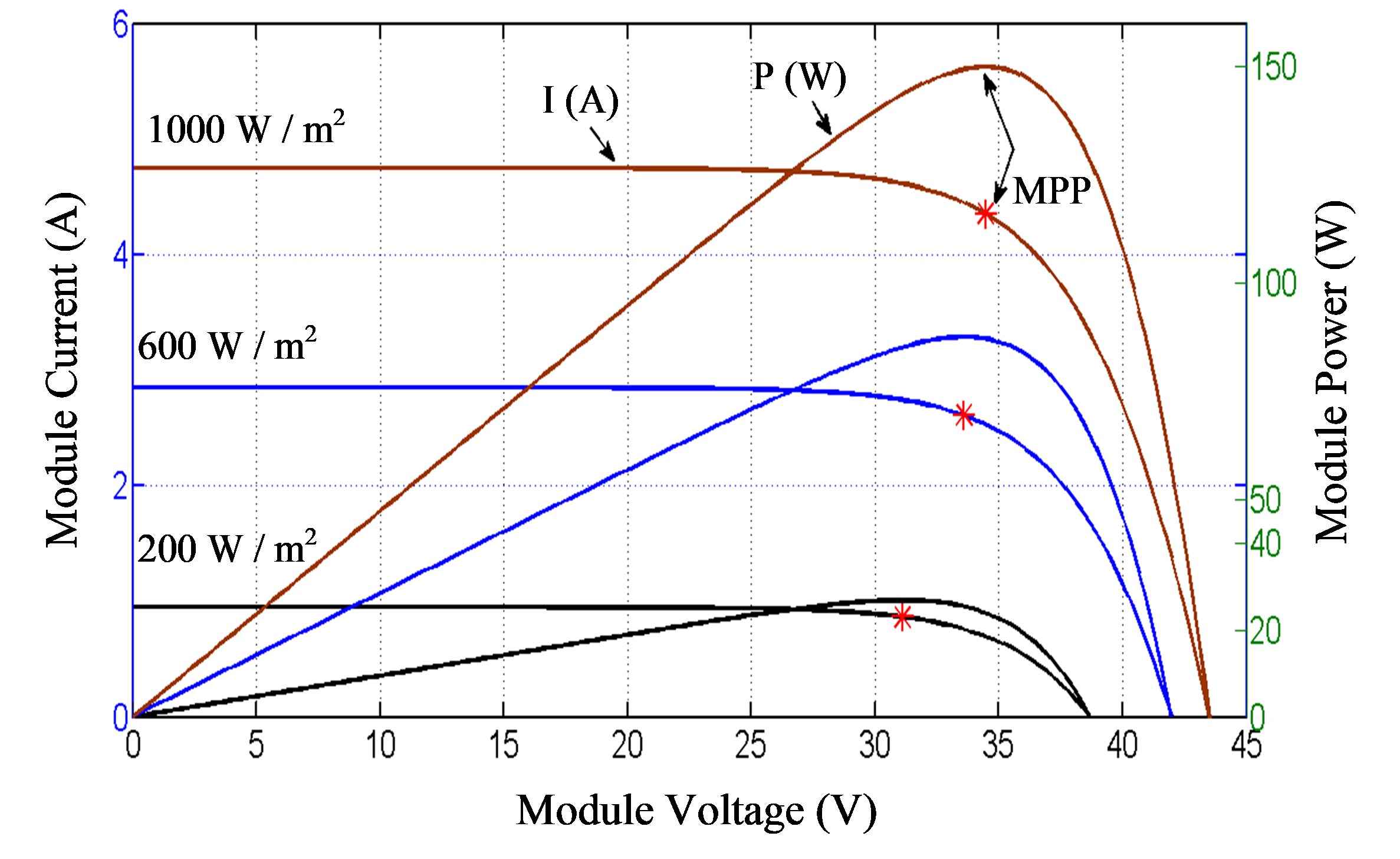Figure 3. I-V and P-V Characteristics of the PV module at various irradiations and 25 ^oC of temperature.

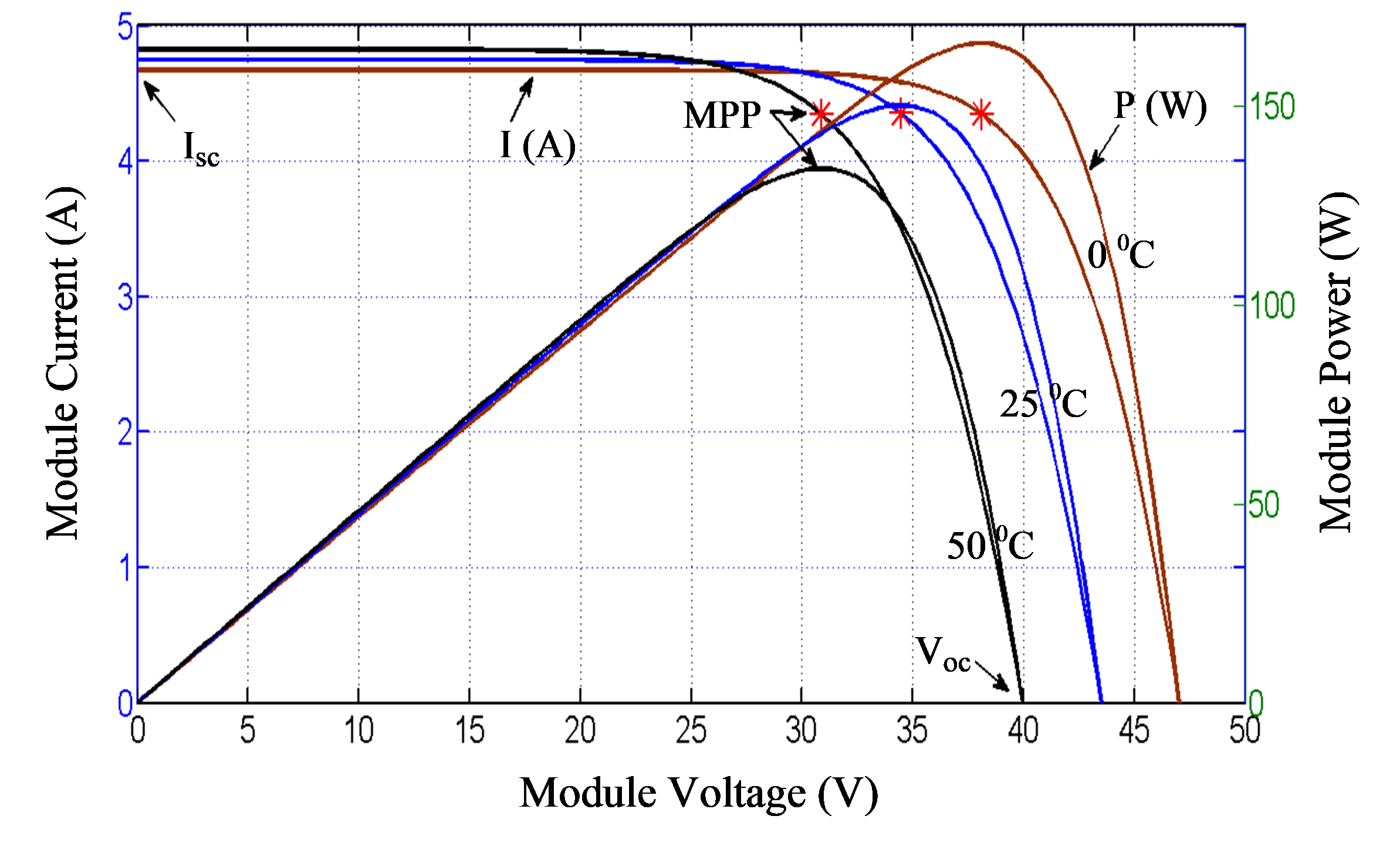Figure 4. I-V and P-V Characteristics of the PV module at various temperatures and 1000 W/m² of irradiation.

3.       MPPT Control and Load Matching

The switch mode DC-DC converter represents a main part of the PV MPPT. The DC-DC converter is used for two purposes; firstly, to regulate the PV operating point at the MPP. Secondly, to maintain the matching between the PV optimal impedance (R_opt) and the connected load impedance (R_L), consequently, a maximum power transfer between the PV module and the load can be obtained. The DC-DC converter uses the duty cycle control signal produced by the MPPT algorithm [1].

According to an ideal (lossless) DC-DC converter, the input-output voltage and current relationships can be described by:

Where, V_L and I_L are the load’s voltage and current, respectively. Whereas V and I are the PV module’s voltage and current, respectively. The relationship between the voltage and duty cycle can be expressed as:

• If 0 < D < 0.5, the converter output voltage does not exceed the input voltage (Buck type).
• If D = 0.5, the converter’s input and output voltages are identical.
• If 0.5 <D < 1, the converter output voltage exceeds the input voltage (Boost type).

The DC-DC converter’s input impedance (i.e. input impedance seen by the PV module) can be written as:

 From (10), it can be seen that by changing the duty cycle, the value of R_in can be matched with the optimal input impedance (R_opt) of the PV module at the MPP, where,

At STC, the relationship between the duty cycle and extracted power from the PV module at various values of resistive load (R_L) is shown in Figure 5 [1]. As it is seen in this figure, when R_L is increased, the optimal duty cycle (D_opt) is also increased to reach the unique MPP. In this paper, the goal of the two utilized MPPT methods is to maintain D_opt under various climate (G and T) conditions and resistive load (R_L).

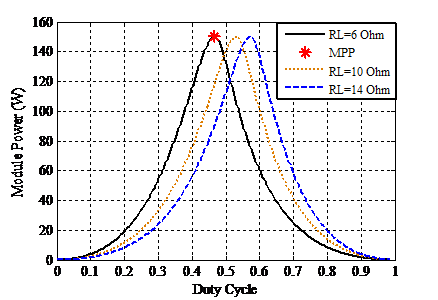Figure 5. Module power vs. duty cycle at STC and various resistive loads.

4.       MPPT Algorithms

4.1.  Perturb and Observe (P&O) Method

The perturb and observe (P&O) method, also known as the “hill climbing” method is widely used as an MPPT algorithm for PV systems applications due to its simplicity and ease of implementation and simplicity [11]. The algorithm perturbs the duty cycle by increasing or decreasing it using a constant duty step-size (ΔD) and observes resulting variations in the PV output power (ΔP). If the ΔP˃0, that means the new operating point has moved closer towards the MPP, hence the duty cycle is further perturbed in the same direction; otherwise, the direction will be reversed. This process is repeated periodically until MPP is maintained. Unfortunately, by this algorithm, the operating point oscillates around the MPP at the steady state. Consequently, the PV efficiency is slightly reduced. Although the steady state oscillation can be decreased by decreasing ΔD, however, the dynamic response will be slowed. Hence, the tradeoff between these two requires that ΔD is finely tuned. The flow chart of the P&O algorithm is shown in Figure 6.

Figure 6. Flow chart of the P&O algorithm.

4.2.  Fuzzy Logic Control (FLC) Method

The fuzzy logic was developed by Zadeh in 1965. The FLC is used to convert the human information to the rule-based model that can control a plant with linguistic explanations [12,13].

In this paper, the utilized FLC has two inputs and one output. The inputs are an error (E) and its variation (ΔE), whereas the output is the change in duty cycle (ΔD), as shown in Figure 7.

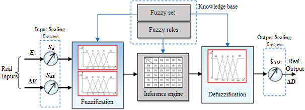Figure 7. The Structure of a fuzzy logic controller.

The inputs and output, at a sampling instant k are expressed as follows:

Where P(k) and V(k) are the output power and voltage of the PV module at sampling k. ΔD(k) is the change in duty cycle used as the FLC’s output to calculate the DC-DC converter’s actual duty cycle D(k) at sampling k.

E(k) is the P–V curve’s slope. Consequently, the sign of E(k) indicates the operating point’s location at instant k, either on the left or on the right of the MPP on the P–V curve of PV module as illustrated in Figure 8. However, the input ΔE(k) expresses the moving direction of this point. The typical FLC includes three main components: fuzzification, inference engine, and defuzzification, as shown in Figure 7 [14].

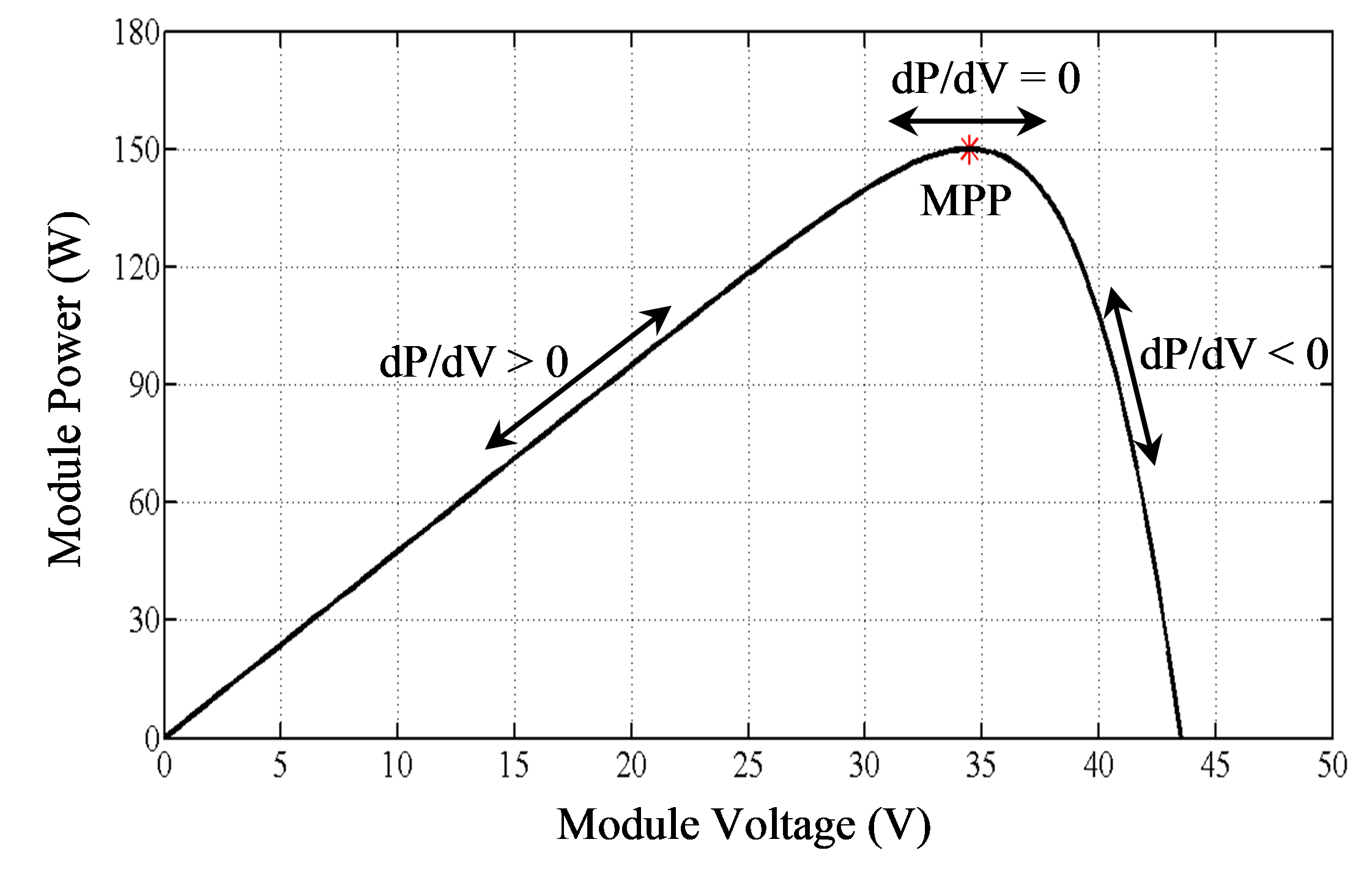Figure 8. The slope of P–V characteristics of PV module at STC.

I. Fuzzification

After normalizing the actual (crisp) FLC’s inputs by scaling factor (S_E) and (S_ΔE), as shown in Figure 7, the inputs are fuzzified. The fuzzification process converts the input and output variables from real crisp variables to fuzzy variables which are expressed by linguistic terms such as negative big (NB), negative small (NS), zero (Z), positive small (PS), and positive big (PB). Figure 9 shows the fuzzy sets for the inputs and output variables used in this paper with triangular and trapezoidal membership functions.

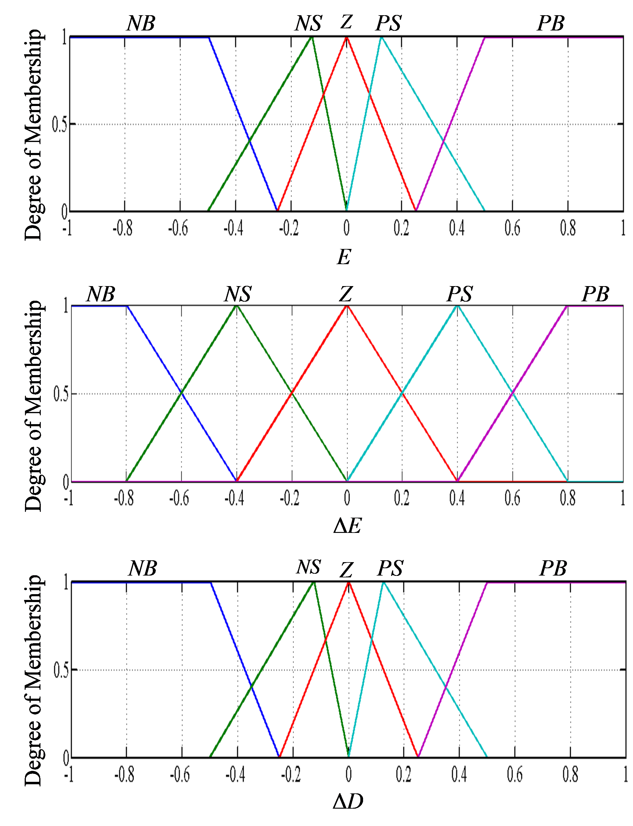Figure 9. Membership functions: E and ΔE are the inputs; ΔD is the output.

II. Fuzzy Rules and Inference Engine

The inference engine applies the rules to the fuzzy inputs which are produced by the fuzzification process to generate n aggregated fuzzy outputs. In this paper, since each of the input and output has five fuzzy subsets, 25 fuzzy IF-THEN rules shown in Table 2 are used. The rules are used to control the DC-DC converter by a suitable ΔD.

The main concept of the rules is related to the location of the operating point from the MPP. If the operating point moves closer toward the MPP, the ΔD will be increased or decreased to a small extent and vice versa if the operating point diverges away from the MPP. For example, in the shaded rule in Table 2: If E is NB AND ΔE is Z THEN ΔD is PB. This means that if the operating point is located at a distance to the right of the MPP and there is no change in the P–V slope, then the duty ratio is substantially increased.

Table 2. Fuzzy logic controller rules

ΔD		ΔE
		NB	NS	Z	PS	PB
E	NB	Z	Z	PB	PB	PB
	NS	Z	Z	PS	PS	PS
	Z	PS	Z	Z	Z	NS
	PS	NS	NS	NS	Z	Z
	PB	NB	NB	NB	Z	Z

III. Defuzzification

The defuzzification represents the inverse of the fuzzification process. It is used to transform the output from the fuzzy domain into the single real (crisp) domain, using the well-known center of gravity (COG) defuzzification methods. This method computes the centroid of the final composite area representing the output fuzzy term, which is resulted by the union of all 25 rule output fuzzy sets [15,16], to produce the real value of ΔD as:

Finally, this crisp output is denormalized using the output scaling factor (S_ΔD) then substituted in (15) to generate the actual duty cycle D(k).

5.       Simulation Results

In this paper, the load, irradiation, and temperature variations are presented in Figures 10–12, respectively.

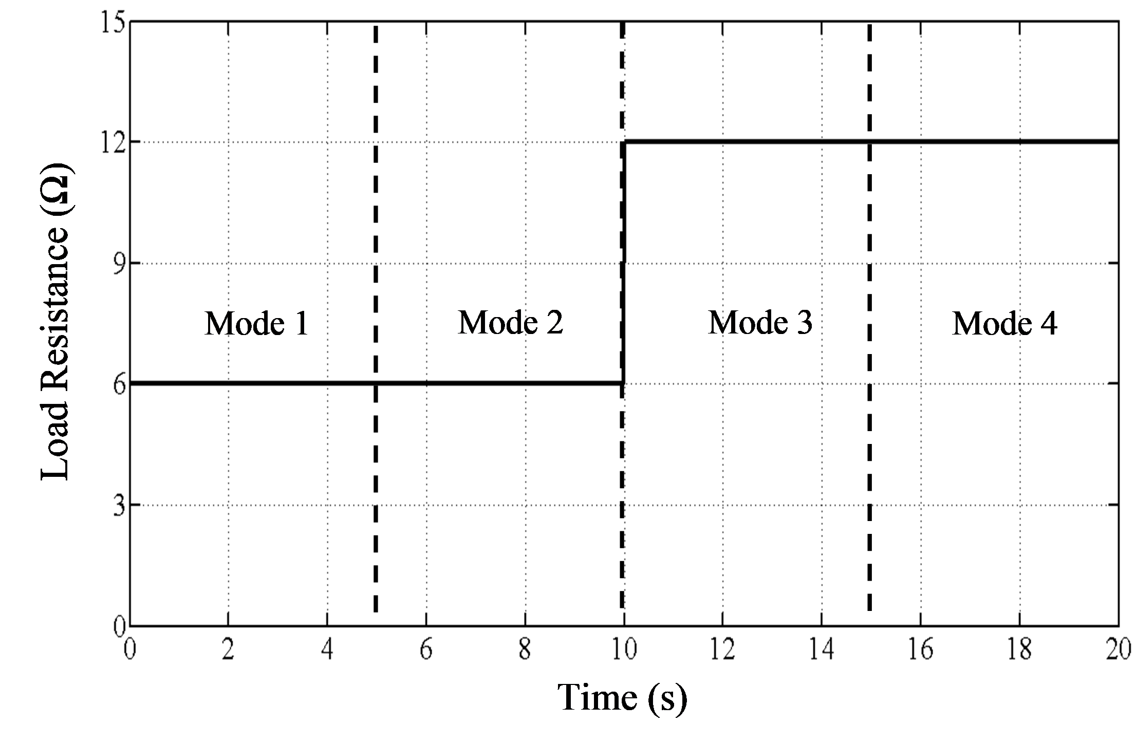Figure 10. Resistive load variation.

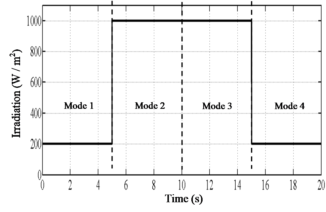Figure 11. Irradiation variation.

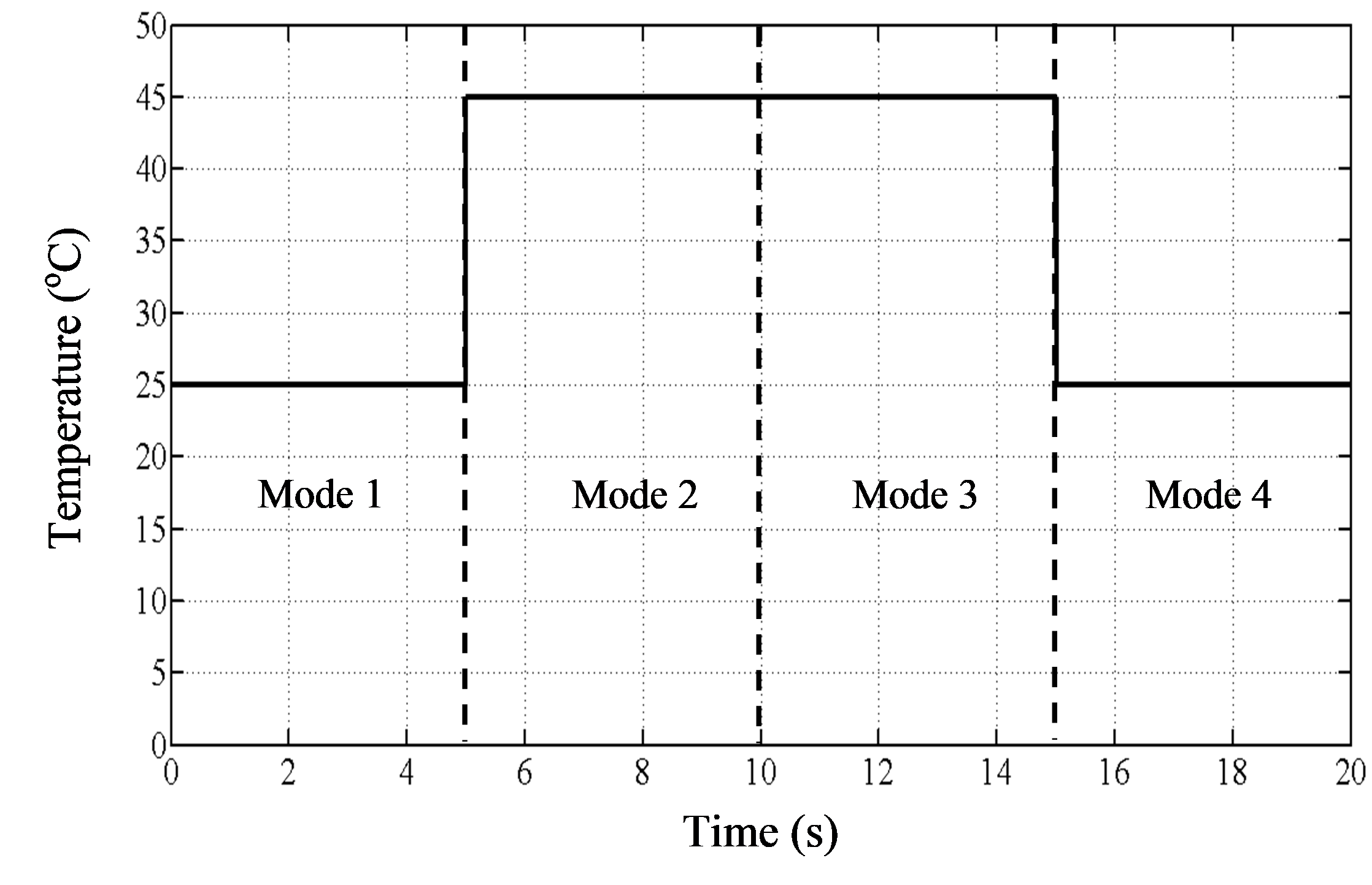Figure 12. Temperature variation.

The overall operating period can be classified into four different modes:

• Mode 1 is the period where G=200W/m², T=25 ^oC, and R_L=6 Ω.
• Mode 2 is the period where R_L is kept constant whereas G and T are suddenly increased to 1000W/m² and 45 ^oC, respectively.
• Mode 3 is the period where the load is changed from 6Ω to 12 Ω at constant G and T of the previous
• Mode 4 is the period where the load is kept constant whereas G and T are suddenly decreased to the same its values in mode 1.

During the time period of mode 1 shown in Figures 10–12, the MPPT methods increase the duty cycle from initial value (D=0.1) to (D_opt1=0.29), as shown in Figure 13 and decrease the converter input resistance (R_in) by using (10) to match (R_opt1=35.92 Ω), moving the operating point of the PV module from starting point A to reach MPP at point B, as shown in Figure 14, thereby extracting maximum power (P_max1=27 W) from the module as shown in Figures 15–17.

Due to a large increasing in the irradiation at the starting mode 2, the operating point will suddenly jump to point C, as shown in Figure 14 with a small increasing in power to (P=40 W), as shown in Figures 15–17. During this mode, the MPPT methods increase D to (D_opt2=0.476), as shown in Figure 13 and decrease R_in to match the new (R_opt2=7.27 Ω), moving the operating point from point C to the new second MPP at point D, as shown in Figure 14, thereby increasing the power to (P_max2=137.3 W), as shown in Figures 15–17.

At the starting of mode 3, when the load is suddenly doubled, R_in is also doubled from 7.27 Ω to 14.54 Ω, thus the operating point will suddenly jump away in the right direction from point D to point E, as shown in Figure 14 and the power drops from P_max2 to 95 W, as shown in Figures 15–17. During this mode, the tracking methods try again to recover the operating point from current point E to the MPP at point F which is the same location of optimal point D, by moving it in the left direction, by increasing D from D_opt2 to new (D_opt3=0.5624), as shown in Figure 13 and decreasing R_in to match R_opt2 again, as shown in Figure 14, to reach P_max2 again, as shown in Figures 15–17.

Finally, at the starting of mode 4, when the load is kept constant and the climate conditions drops as the inverse of starting condition of mode 2, the operating point will suddenly jump to point G shown in Figure 14 with a large decreasing in power from P_max2 to 7.5 W, as shown in Figures 15–17. During this period, the MPPT methods decrease D to (D_opt4=0.3663), as shown in Figure 13 and increase R_in to match (R_opt1=7.27 Ω) again, moving the operating point in the right direction from point G to the MPP at point H which is the same location of optimal point B, as shown in Figure 14, thereby increasing the power and reaching P_max1 again_, as shown in Figures 15–17.

From the different operation modes, it is clear that the FLC provides a fast and effective transient response in terms of tracking and recovering speed and this method also provides an effective steady response with less oscillation as compared with P&O tracking method, according to the responses of duty cycle and extracted power from the PV module shown in Figures 13, 16, respectively.

At variable climate and load operation modes explained in Figures 10–12, Table 3 lists the load matching results of voltage, current, and power of PV module, duty cycle and input resistance of the DC-DC converter, and the corresponding load voltage and current using MPPT.

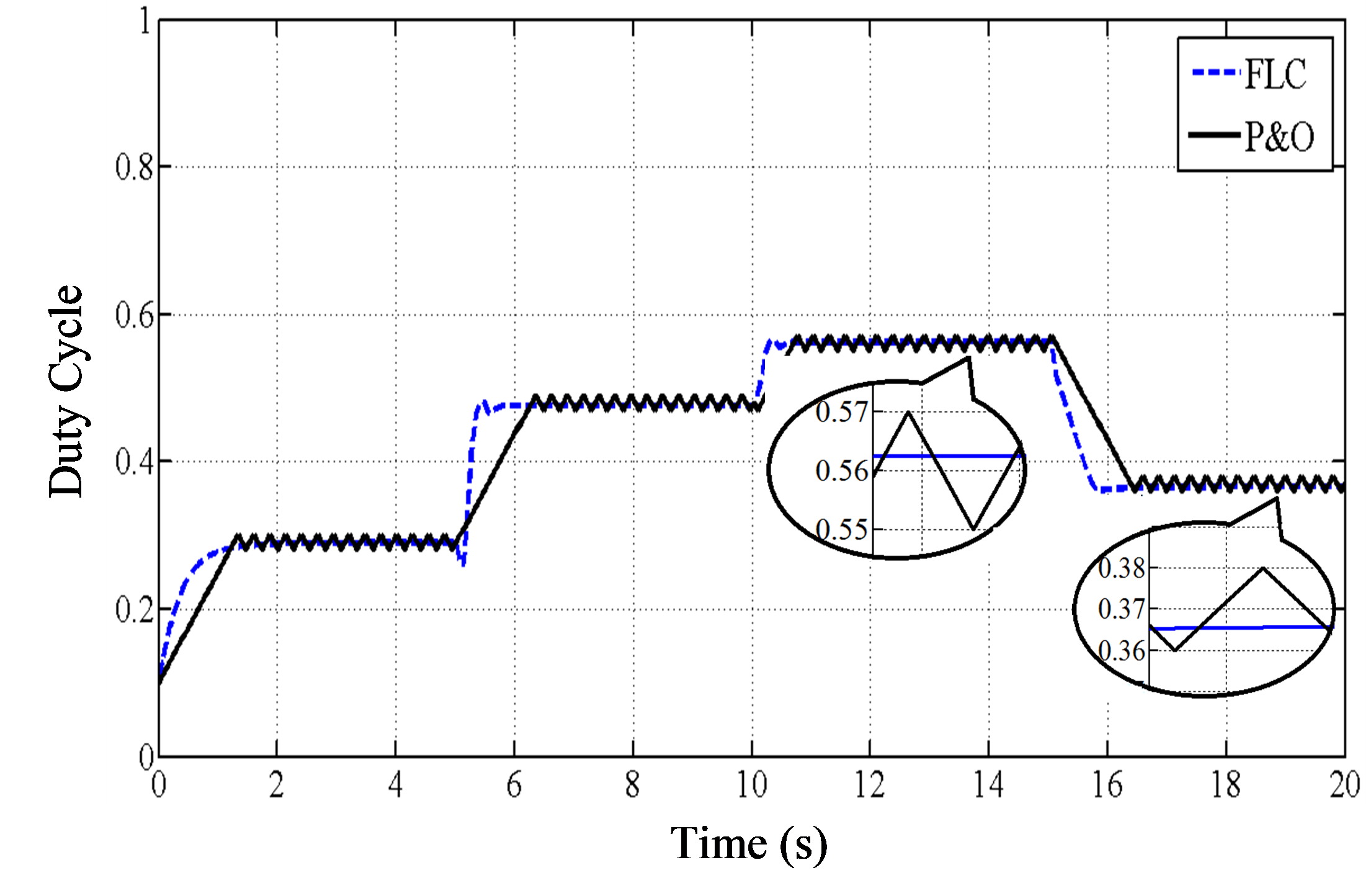Figure 13. Duty cycle performance using MPPT methods under variable climate and load conditions.

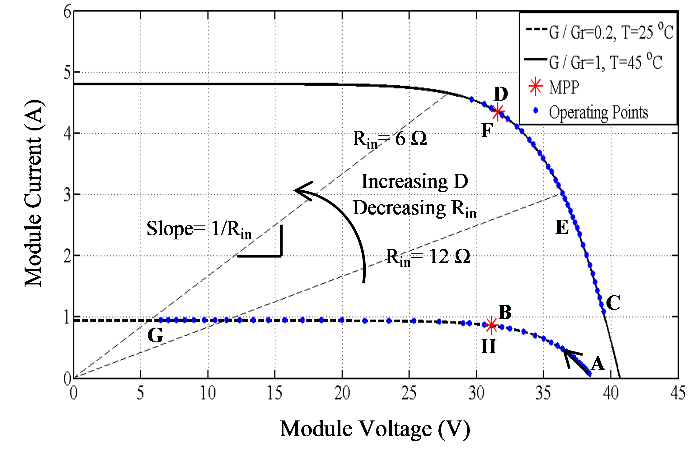Figure 14. I–V Characteristics of PV module and traces of operating point under variable climate and load conditions.

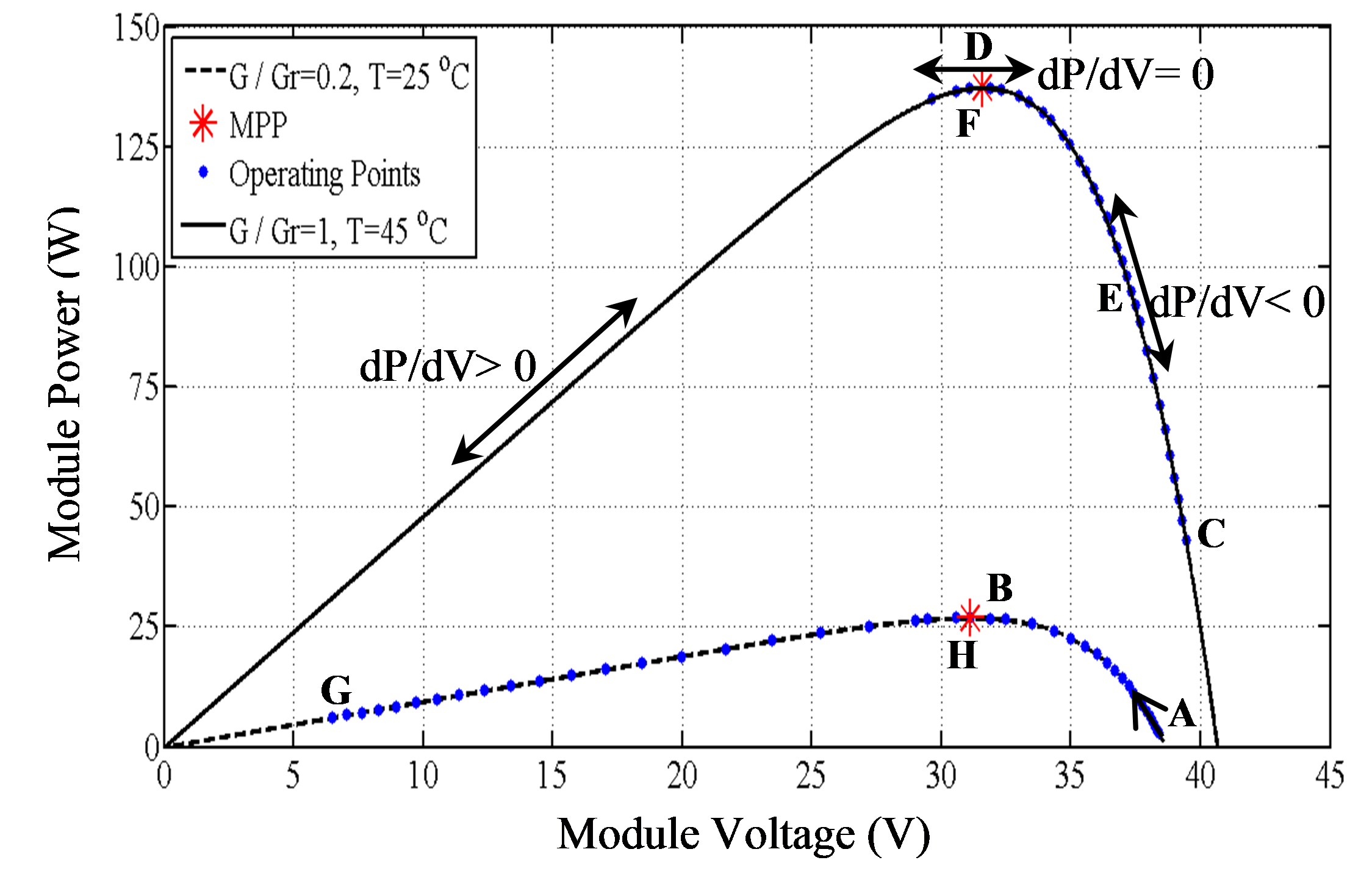Figure 15. P–V Characteristics of PV module and traces of operating point under variable climate and load conditions.

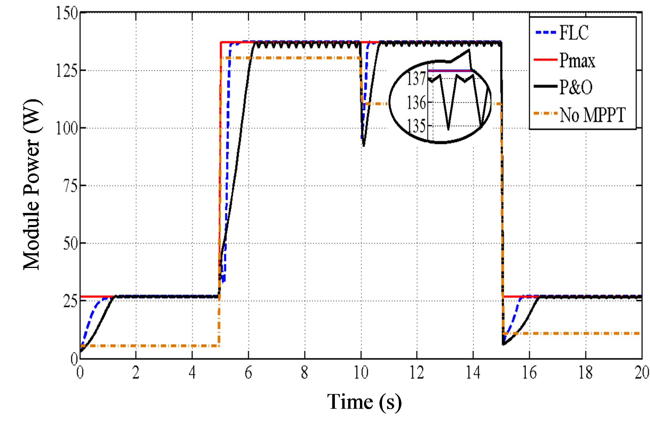Figure 16. Module power performances using MPPT methods under variable climate and load conditions.

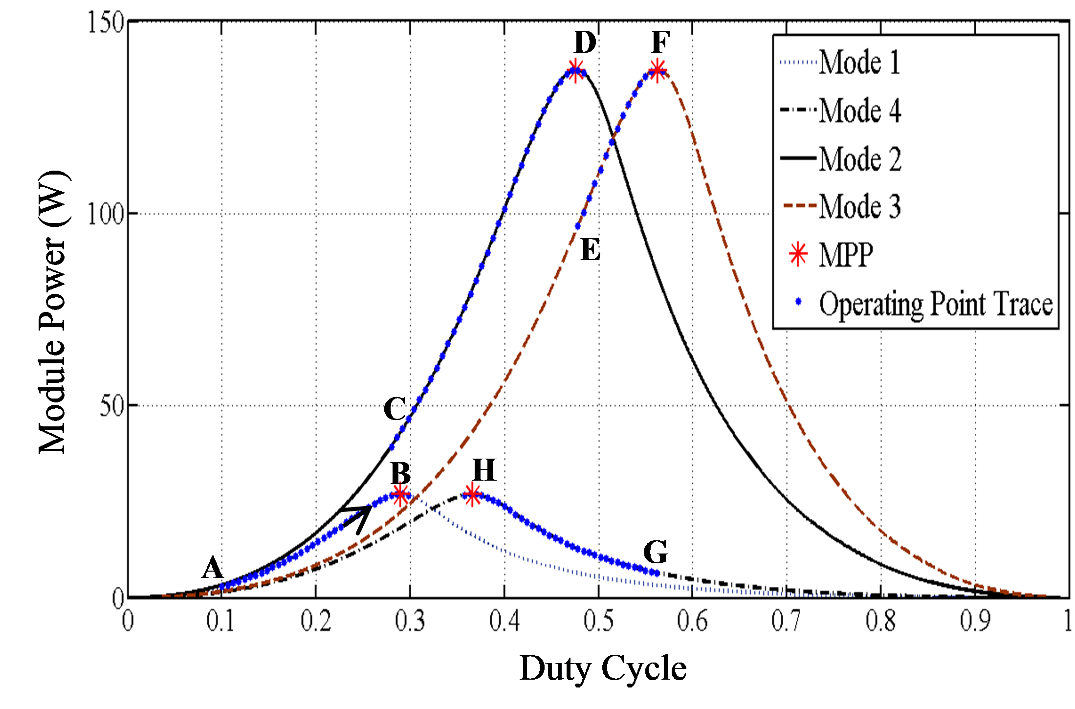Figure 17. Module power vs duty cycle and traces of operating point under variable climate and load conditions.

Whereas, Table 4 lists the comparison results of MPPT methods in terms of rising time, recovery time, total average power, and MPPT efficiency during the overall operating period.

Table 3. Load matching results under different operating modes

Operating Modes	Vmpp (V)	Impp (A)	Pmax (W)	Ropt (Ω)	Dopt	Vo (V)	Io (A)
Mode 1	31.1	0.86	26.92	35.92	0.29	12.71	2.12
Mode 2	31.6	4.34	137.3	7.27	0.47	28.70	4.34
Mode 3	31.6	4.34	137.3	7.27	0.56	40.59	3.38
Mode 4	31.1	0.86	26.92	35.92	0.36	17.97	1.49

Table 4. Comparison of MPPT methods under different operating modes

MPPT Method	t r (s)	Recovering Time (s)	Ideal Pav (W)	Total Pav (W)	Efficiency %
Without (D=0.5)	–	–	82.1137	64.153	78.12
P&O	1.25	0.75	82.1137	76.3	92.92
FLC	0.75	0.25	82.1137	79.66	97.01

6.       Conclusions

In this paper, the effectiveness of the FLC and classical P&O based MPPT methods are analyzed by simulation and compared using different operation modes of irradiation, temperature, and load requirement.

In the case of rapid changes in the climate conditions and constant connected load, as represented by starting periods of modes 2 and 4, the simulation results show that the FLC tracking method can quickly reach the new MPP with less rising time (t_r) at transient response and eliminates the power oscillation around the MPP at steady state; thus providing a higher power output efficiency, as shown in Figures 13, 16 and Table 4.

According to a rapid fluctuation of the load, as represented by starting periods of mode 3, also the FLC method has better performances in comparison with P&O method – less recovering time and better steady responses of less oscillation as shown in Figures 13, 16 and Table 4. Consequently, the PV system with FLC-based MPPT control is more efficient due to the fact that allows harvesting more solar power in comparison with the classical P&O tracking methods.

Acknowledgment

The first author thanks ‎the ‎‏Iraqi government represented by the Ministry of higher education and scientific research, Al-Mustansiriya University, Baghdad, Iraq for its financial support.

1. A. G. Al-Gizi, “Comparative study of MPPT algorithms under variable resistive load” in Proc. of the IEEE International Conference on Applied and Theoretical Electricity (ICATE 2016), Craiova, Romania, 2016. doi: 10.1109/ICATE.2016.7754611
2. V. M. Elena and Papadopoulou, Photovoltaic Industrial Systems: An Environmental Approach, Green Energy and Technology, Springer Heidelberg Dordrecht, London-New York, 2011.
3. F. L. Tofoli, D. Pereira, W. Josias, “Comparative study of maximum power point tracking techniques for photovoltaic systems” International Journal of Photoenergy, 2015, 1–10, Jan. 2015. doi: 10.1155/2015/812582
4. S. Z. Hassan, H. Li, Y. H. Liu, T. Kamal, U. Arifoglu, S. Mumtaz, L. Khan, “Neuro-fuzzy wavelet based adaptive MPPT algorithm for photovoltaic systems” Energies, 10(3), 1–16, 2017. doi: 10.3390/en10030394
5. P. C. Cheng, B. R. Peng, Y. H. Liu, Y. S. Cheng, J. W. Huang, “Optimization of a fuzzy-logic-control-based MPPT algorithm using the particle swarm optimization technique” Energies, 8(6), 5338–5360, 2015. doi: 10.3390/en8065338
6. C. L. Liu, J. H. Chen, Y. H. Liu, Z. Z. Yang, “An asymmetrical fuzzy-logic-control-based MPPT algorithm for photovoltaic systems” Energies, 7(4), 2177–2193, 2014. doi: 10.3390/en7042177
7. T. Salmi, M. Bouzguenda, “Matlab/Simulink based modeling of solar photovoltaic cell” International Journal of Renewable Energy Research, 2(2), 2012.
8. V. V. Naidu, T. M. Mohan, “Modeling and simulation of photovoltaic system” Golden Research Thoughts, 3(6), 1–6, 2013.
9. M. Spasoje, M. Nedeljkovic, “The solar photovoltaic panel simulator” Rev. Roum. Sci. Techn. – Électrotechn. Et Énerg, 60(3), 273-281, 2015.
10. http://www.abcsolar.com/pdf/bpsx150.pdf
11. M. T. Makhloufi, M. S. Khireddine, Y. Abdessemed, “Maximum power point tracking of a photovoltaic system using a fuzzy logic controller on dc-dc boost converter” IJCSI International Journal of Computer Science, 11(3), 1694–0784, 2014.
12. A. V. Pavan, A. M. Parimi, K. U. Rao, “Implementation of MPPT control using fuzzy logic in solar-wind hybrid power system” in Proc. of the IEEE International Conference on Signal Processing, Informatics, Communication and Energy Systems (SPICES), Kozhikode, India, 2015. doi: 10.1109/SPICES.2015.7091364
13. A. M. Othman, A. Fathy, A. Ghitas, “Realworld maximum power point tracking simulation of PV system based on fuzzy logic control” NRIAG Journal of Astronomy and Geophysics, 186–194, 2012. doi: 10.1016/j.nrjag.2012.12.016
14. B. Bendib, F. Krim, H. Belmili, M. F. Almi, S. Boulouma, “Advanced fuzzy MPPT controller for a stand-alone PV system” Energy Procedia, 50, 383–392, Dec. 2014. doi: 10.1016/j.egypro.2014.06.046
15. A. G. Al-Gizi, A. Craciunescu, S. J. Al-Chlaihawi, “The use of ANN to supervise the PV MPPT based on FLC” in Proc. of the 10th IEEE International Symposium on Advanced Topics in Electrical Engineering (ATEE), Bucharest, Romania, 703–708, 2017. doi: 10.1109/ATEE.2017.7905128
16. S. Z. Hassan, H. Li, T. Kamal, M. Nadarajah, F. Mehmood, “Fuzzy embedded MPPT modeling and control of PV system in a hybrid power system.” In Emerging Technologies (ICET), 2016 International Conference on, pp. 1-6. IEEE, 2016. doi: 10.1109/ICET.2016.7813236

(Click to view)

(Click to view)