1. Introduction

There are several methods to derive a mathematical model for a motion process from time series data. In mathematical models directly derived from observed data, the relation among only time series data describes a state value Z; the other state variables are not essential to describe the motion process. The auto-regression (AR) model is well known as a mathematical model to describe Gaussian time series with distributions that are regarded as normal. This mathematical model has succeeded in describing various stationary processes. However, there are currently no established methods to derive a mathematical model directly from non-Gaussian time series data for the sway of the center of gravity of a human body [1], meteorological elements [2], or exchange rates of JP¥ to US$ [3]. Moreover, it is difficult to extract hidden variations in the state variables that are not directly observable. We propose a method to construct stochastic differential equations (SDEs) describing the non-Gaussian processes in stationary states and to obtain a static potential function in the meaning of the temporal average.

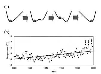
In recent years, it has been suggested that the potential function changes temporally through some analysis of climatic change. Air temperature has shown an upward tendency in statistical tests in previous research [4]. These tests were reasonable to show a general tendency; however, these were insufficient to analyze details of the temporal variations. Shimizu and Takada [2] found temporal variations in the form of histograms on which a new peak appears at higher temperature and variations in form of the potential function in the meaning of the temporal average, which is derived from the form of the histogram in agreement with Takada et al. [1]. The authors have proposed that variations in the form of the potential function are assumed to follow a delay convention of one-dimensional cut off of the wedge catastrophe [5]. If the same type of conventions were introduced into the temporally averaged potential, we could build up the following hypothesis involved in the physical system describing a climatic change as seen in air temperature.

Hypothesis A stationary point of the temporally averaged potential moves in agreement with a delay convention (Figure 1a) in catastrophe theory.

Assuming that these assumptions are satisfied, we can give a physical explanation of time series; for example, a downward arrow in Figure 1b indicates the appearance of a stable equilibrium point of high temperature in the 1990s. Moreover, this hypothesis gave us an opportunity to find a transition of the temporally averaged potential function. It was suggested that there are transition and temporal variations in the temporally averaged potential function caused by breaches of stationary states. There may be dynamic potentials depending on time in contrast to the static potential functions that we have constructed. The author believes that it is often the complexity seen in these systems that controls the biomaterial and living bodies. In this study, we focus on the system that controls the upright posture in the human body.

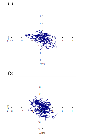
The center of pressure (COP) on the Euclid space E² ∋(x, y) is measured as a time series that comprises the stabilograms (Figures 2 and 3). The time series of sways in stabilograms in the lateral (x) and anterior–posterior (y) directions can be assessed independently [6, 7]. The SDEs

are used as mathematical models to describe sways of the COP [1, 8-10]. Here, w_x(t), w_y(t) are white noise terms and U_x and U_y express their temporally averaged potential functions. In a previous study, the body sway was described by the Brownian motion in which U_x and U_y are expressed by parabolic functions [8-10]. In the last two decades, the limitations of this stochastic process have been realized by [1, 11, 12]. In the following section, we state a methodology to construct the temporally averaged potential functions based on the time series data.

2. Theory

In general, various stochastic processes are expressed by nonlinear SDEs for a random variable z(t):

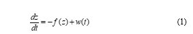
where  indicates white noise and  is a nonlinear function. This SDE has already been applied to describe some time series data mentioned above. In particular, we suggest a method to construct an SDE as a mathematical model for these non-Gaussian time series data as follows.

Assumption 1. We assume that  is one of the Markov processes that is determined by  and .

Assumption 2. We assume that is not an anomalous process that extends far rapidly in a short time.

Based on these assumptions, a stochastic process can be described by a Fokker–Planck equation (FPE). The FPE is rewritten as follows for the distribution of the random variable :

by a change of variables to normalize the second term of the FPE [13], called FPE normalization. Here,  indicates a conditional probability at time  in the initial condition of . As Eq. (2) is a FPE, it does not have a coefficient function depending on the random variable  in the second term. This FPE uniquely corresponds to the SDE by calculating the moment of the transition probability for degree n (n = 1,2,3,…). Taking the average of both sides of Eq. (1) for any stationary interval K, one can obtain the following integro-differential equation:

In the meaning of the time average, the ordinary differential equation (ODE)  is satisfied. Thus, there is a good possibility that the mean values are controlled by the ODE. The curved surface  is regarded as an equilibrium space for the SDE in the meaning of the temporal average (a temporally averaged equilibrium space), and the space integral of the function

is defined mathematically as a temporally averaged potential function. In fact, the potential function in the SDE seems to fluctuate; the potential function cannot strictly be obtained in a certain time. The authors thus considered the potential function to be a fluctuating potential.

A stationary solution  to the FPE (2) has been found under a natural boundary condition [14]. Under Assumptions 1 and 2, the author pointed out that it was important to analyze the forms of the histograms corresponding to the temporally averaged potential functions as

because the stationary solution could be regarded as a density distribution through a long observation. We then regarded the stationary solution (a probability density function) as a density distribution, which is the normalized histogram of the time series data. That is, one can estimate the SDE as a mathematical model for time series data using Eq. (5). However, it is necessary to estimate a formula as a temporally averaged potential function from the standpoint of the numerical analysis. To approximate the temporally averaged potential function, we fit polynomials of degree  to the logarithmic density distribution under the following demands.

• Demand on statistics: The coefficients of determination for the optimal polynomial fitting to the logarithmic density distribution must be greater than 0.9.
• Demand on geometry: The potential function should be structurally stable taking into consideration the perturbation exerted on the control system.

3. Materials and Methods

Thirty-two healthy subjects voluntarily participated in the study; all of them were Japanese and lived in Nagoya and its environs. They were divided into two groups: a group of young people aged less than 22 years (20 ± 1 year) and a group of elderly people aged more than 65 years (70 ± 4 years). Each group included the same number of subjects. The following were the exclusion criteria for subjects: subjects working in a night shift, subjects with dependence on alcohol, subjects who consumed alcohol and caffeine-containing beverages after waking up and meals within two hours, subjects who may have had any otorhinolaryngologic or neurological disease in the past, except for conductive hearing impairment, which is commonly found in the elderly. The subjects were not prescribed drugs for any disease by doctors. The local ethics committee of the Nagoya University School of Health Science approved this study (approval number 7-129), and the subjects gave their informed consent prior to participation.

In the subsequent stabilometric analysis, we recorded the COP at rest and during GVS. We ensured that the body sway was not affected by environmental conditions; using an air conditioner, we adjusted the temperature to 25 °C in the exercise room, which was large, quiet, and bright. All subjects were tested from 10 am to 5 pm in the room of Nagoya University; they were positioned facing a wall on which a visual target was placed; the distance between the wall and subjects was 2 m.

Before the sway was recorded, the subjects stood still for 1 min in the Romberg posture with their feet together on the detection stand of a stabilometer (G5500, Anima Co., Ltd.). The COP sway was recorded (sampling frequency: 20 Hz) when the subjects stood with their eyes open (1 min) and looked at a visual target placed at a distance of 2 m or when their eyes were closed (subsequent 1 min). The stabilograms were simultaneously recorded using the stabilometer.

Every second, rectangular current impulses were output from an electronic stimulator (SEN-3301, Nihon Kohden Co., Ltd.). The duration of the current was set to 0.5 s. A small electric current (0.6–2.0 mA) was percutaneously applied to both sides of the mastoid processes through Ag/AgCl electrodes of an isolator (SS-104J, Nihon Kohden Co., Ltd.). We set the amplitude of the electric current to the maximum value obtained in the following anti-GVS test [15]; this value varied among subjects.

4. Results

Stabilometry was performed with subjects standing on stabilometer in the case of the resting state (Figures 2). Then, the

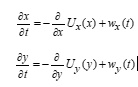
anti-GVS test was employed to the young and elderly subjects, and stabilograms were recorded during the GVS (Figures 3). In these figures, the vertical axis shows the anterior and posterior movements of the COP, and the horizontal axis shows the right and left movements of the COP. The amplitudes of the sway that was observed in the elderly subjects tended to be larger than those of the sway that was observed in the young subjects (Figures 2-3). Furthermore, the lateral movement of the COP was often observed during the GVS shown in Figures 3.

The amplitudes of the sway are affected by electric current during periodic GVS. It is considered that a periodic function s(t) is added to the SDE as a forcing term, and the form of the potential function U(z) changes [15]. The effective potential is expressed as

where z is a space variable in the lateral direction x, that is, the direction of the GVS-evoked body sway. Using the sparse density [7] in the analysis of stabilograms, we investigate the evolution of the potential function U(z) in this study. By comparing the stabilograms, we study the effects of aging and GVS on the sway of the COP.

5. Discussion

The nonlinear property of SDEs is important although the concept of simple muscle stiffness control during quiet standing has been accepted for a long time [16, 17]. However, the linear model [8–10] has been rejected by the experimental results of the relationship between the body posture angle and the ankle torque [18, 19], and the postural instability, which is called “microfall” [20]. The nonlinear property has also been found in the distribution of the COP [1].

A certain type of standardization is required to provide a mathematical model in accordance with the theory stated in Section 2 because the noise amplitude is set to be 1 in Eq. (1). To prevent arbitrariness in the standardization for each component, we discuss and propose a new scheme using

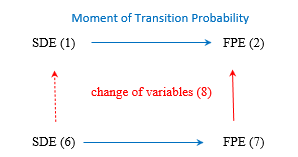
as a mathematical model of the time series in this section. By calculating the moment of the transition probability for degree , this SDE corresponds to

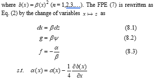
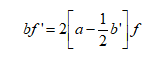
for FPE normalization (Figure 4). Actually, Eq. (2) does not have a coefficient function depending on the random variable  in the second term. By this change of variables, the SDE (1) does not, however, correspond to Eq. (6) but corresponds to the following SDE:

where the prime ′ denotes differentiation with respect to the random variable . In the case of   , the SDE (1) obviously corresponds to Eq. (6), and a stationary solution to Eq. (7) can be found as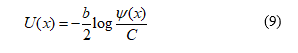

under a natural boundary condition. Otherwise, we should solve the following differential equation:

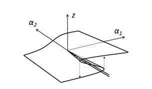
To construct an optimal description (9) for each generator of time series, we fit graphs of polynomials to the logarithmic histogram of the time series, . For example, we herein consider the Riemann–Hugoniot manifold as an equilibrium space (Figure 5). By using Eq. (4), the double-well potential can be extracted from the half line in Figure 5. In general, a polynomial of degree four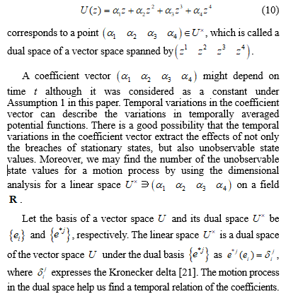 

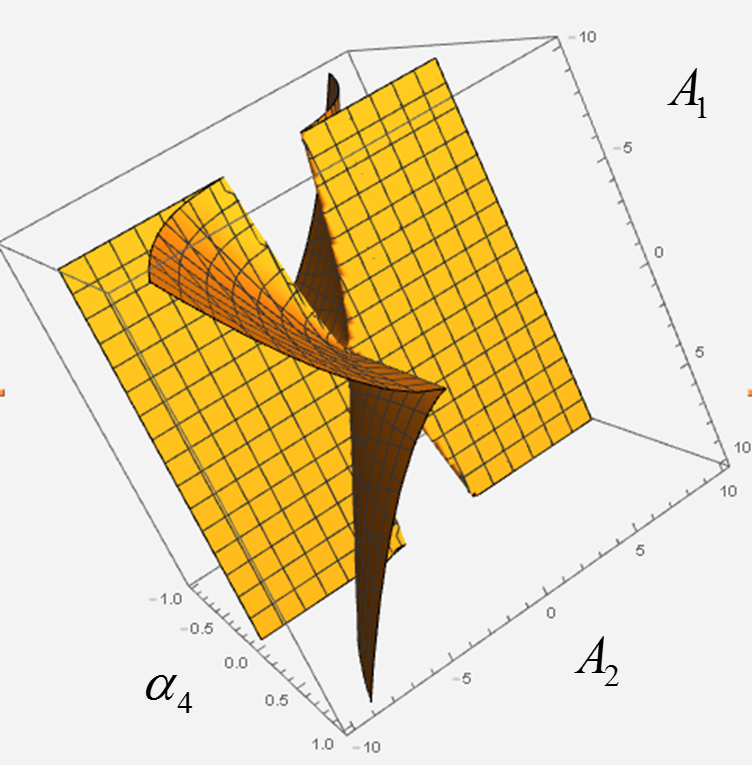
Eliminating the temporal variable , we can look for a mathematical expression of the unobservable state values as an algebraic curve, which is a four-dimensional curve, in the dual space. It is important to study the four-dimensional curve mathematically. If  generated random numbers, the construction method could be applied to sequences  again. We can propose novel potentials in the mathematical models for coefficients of the temporally averaged potential functions or the unobservable state values. In this paper, these novel potential functions are called grand potentials. One can apply the grand potentials to time series analyses for the non-Gaussian and non-stationary processes or forecasts for those motion processes. We may classify strategy for changes of those motion processes on the basis of the grand potentials.

The following translation is useful to simplify the expression of Eq. (10) because the third term on the right-hand side in Eq. (10) goes to zero: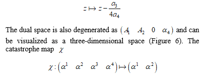

is considered useful for the visualization of the motion process in the dual space. Using the boundary in the dual space (Figure 6), we examine the nonlinearity of the potential during the GVS and the other loads in the next step.

Conflict of Interest

The authors declare no conflict of interest.

Acknowledgment

This work was supported in part by the Japan Society for the Promotion of Science, Grant-in-Aid for Scientific Research (C) Number 26350004.

1. Takada, Y. Shimizu, Y. Kitaoka, “Mathematical index and model in Stabirometly,” Forma, 16 (1), 17-46, 2001.
2. Shimizu, H. Takada, “Verification of air temperature variation with form of potential,” Forma, 16 (4), 339-356, 2001.
3. Takada,”Phase Transition with noise for time series of JP\/US$ exchange rate,” Forma, 31(Special Issue), S41–S53, 2016.
4. IPCC, Greenhouse Gas Inventory, Reporting Instructions, Inter
   -governmental Panel on Climate Change, 1995.
5. Poston, I. N. Stewart, Catastrophe Theory and its Application, Pitman publishing limited, 1978.
6. A. Goldie, T. M. Bach, O. M. Evans, “Force platform measures for evaluating postural control: Reliability and validity,” Arch. Phys. Med. Rehabil., 70, 510–517, 1986.
7. Takada, “A Construction Method of the Mathematical Model on Time Series Data with Markov Property and Verification,” Ph.D. Thesis, Meijyo Univ., 2004. (in Japanese)
8. J. Collins, C. J. D. Luca, “Open loop and closed-loop control of posture: A random-walk analysis of center of pressure trajectories,” Exp. Brain Res., 95, 308–318, 1993.
9. E. A. Emmerrik, R. L. V. Sprague, K. M. Newell, “Assessment of sway dynamics in tardive dyskinesia and developmental disability,” Sway Profile Orientation and Stereotypy. Moving Dis., 8, 305-314, 1993.
10. M. Newell, S. M. Slobounov, E. S. Slobounova, P. C. Molenaar, “Stochastic processes in postural center of pressure profiles,” Exp. Brain Res., 113, 158–164, 1997.
11. Takada, M. Miyao, “Visual fatigue and motion sickness induced by 3D video,” Forma , 27 (Special Issue), S67-S76, 2012.
12. Asai, Y. Tasaka, K. Nomura, T. Nomura, M. Casadio, and P. Morasso, “A model of postural control in quiet standing: Robust compensation of delay-induced instability using intermittent acti-vation of feedback control,” PLoS ONE, 4 (7), art. no.e6169, 2009.
13. S. Goel, and N. Richter-Dyn, Theory of Stochastic Process in Biology, Industrial books, 33-75, 282-287, 1978.
14. Harken, “Cooperative phenomena in systems far from thermal equilibrium and in nonphysical systems,” Rev. Mod. Phys., 47, 67-121, 1975.
15. Takada, M. Takada, K. Tanaka, T. Shiozawa, M. Furuta, M. Miyao, “A simulated study of the deterioration in the equilibrium function with advancing age,” Bulletin of Gifu University of Medical Science 3, 109-117, 2009.
16. A. Winter, A. E. Patla, F. Prince, M. Ishac, K. Gielo-Perczak, “Stiffness control of balance in quiet standing,” J Neurophysio, 80, 1211-1221, 1998.
17. A. Winter, A. E. Patla, S. Rietdyk, M. G. Ishac, “Ankle muscle stiffness in the control of balance during quiet standing,” J Neurophysio, 85, 2630-2633, 2001.
18. D. Loram, M. Lakie, ”Human balancing of an inverted pendulum- position control by small, ballistic-like, throw and catch movments,” J Physioligy, 540, 1111-1124, 2002.
19. D. Loram, C. N. Maganaris, M. Lakie, “Human postural sway results from frequent, ballistic bias impulses by soleus and gastrocnemius,” J Physioligy, 564(1), 295-311, 2005.
20. Bottaro, Y. Yasutake, T. Nomura T., M. Casadio, P. Morasso, “Bounded stability of the quiet standing posture: an intermittent control model,” Human Moving  Science , 27(3), 473-495, 2008.
21. Wadachi, Differential Geometry and Topology, Iwanami, 1996. (in Japanese)

(Click to view)

(Click to view)